
Water quality
EPANET can solve one water quality analysis with the hydraulics, and the app offers all three of them: the age of the water, where the water came from, or what happened to a chemical in it. One setting decides which analysis runs. A run carries one analysis at most. When you choose a new one, it replaces the last one.
No analysis runs by default. If Simulation type was never changed, the model solves the hydraulics only, whatever the assets carry. This page is about where you set up each analysis and where its answer appears. For what each analysis computes, see the EPANET 2.2 manual.
The three analyses
Section titled “The three analyses”| Analysis | What it reports | Unit | What it needs from the model |
|---|---|---|---|
| Age | The time the water at each point spent in the network | Hours | Nothing. The app reads an Initial quality on a source as an age |
| Trace | The share of the water at each point that came from one chosen node | Percent | Trace node |
| Chemical | The concentration of a substance you name | mg/L or μg/L | Sources and the reaction constants |
All three analyses need time to develop, so all three need an extended period run. A steady state run has one moment only, and the water has no time to travel. See Time analysis mode on Simulation settings.
The analysis to run depends on what you want to find out. The water quality simulation model in the EPANET 2.2 manual describes what each one is for:
- Age answers where the water sits too long. Water that enters from a reservoir or a source node starts at an age of zero, and every parcel then ages one second per second. The manual treats the result as a simple, non-specific measure of the overall quality of the water delivered. Age needs no calibrated rate for anything, so it is the one to start with.
- Trace answers which source serves a given area, and how that changes through the day. The case the manual makes is a system that draws on two or more raw water supplies. Trace shows how far the water from one supply blends with the rest, and how the pattern of that blending moves over the run.
- Chemical answers what becomes of a substance on its way through the network. A residual decays, a by-product grows toward a limit, or an inert tracer goes nowhere. Those are the three worked cases of the manual: chlorine as first-order decay, trihalomethanes as first-order growth to a limiting concentration, and a fluoride tracer with no reaction at all. Chemical is the only one of the three that uses the reaction coefficients.
Turning one on
Section titled “Turning one on”Open Simulation settings. Go to Water quality. Set Simulation type. The section has three subsections, and that first row decides what is available in them.
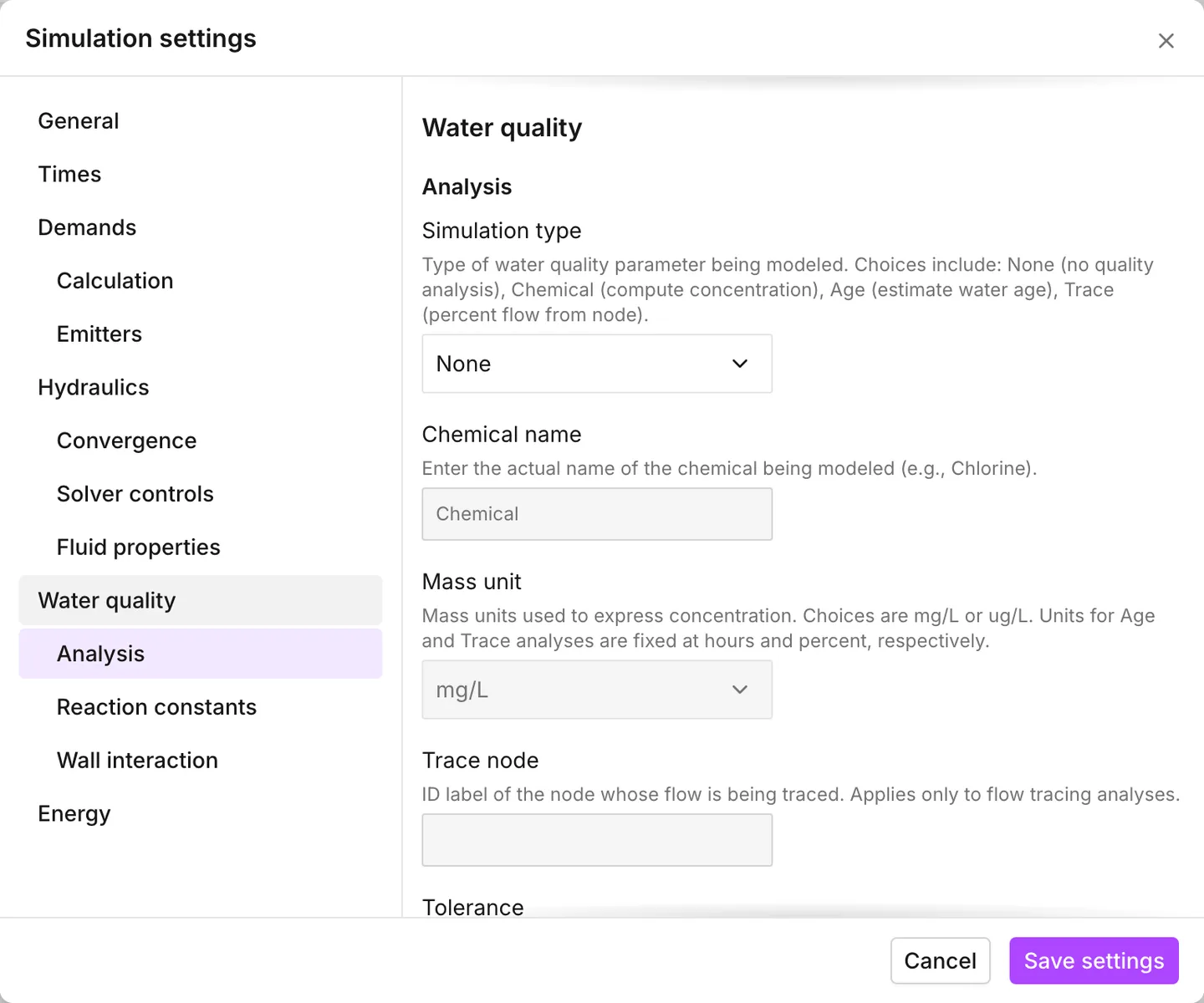
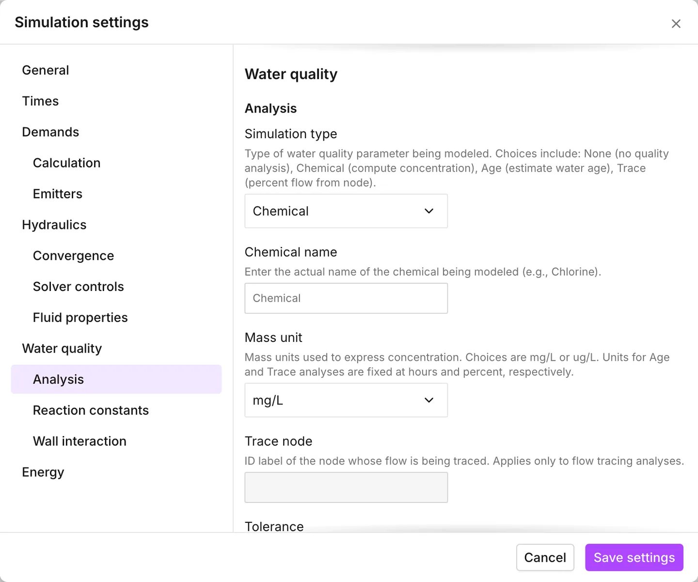
| Row | Available under |
|---|---|
| Simulation type | Always |
| Chemical name, Mass unit | Chemical |
| Trace node | Trace |
| Tolerance | Any analysis other than None |
| Reaction constants and Wall interaction, in full | Chemical |
Trace node takes the label of any node: a junction, a tank or a reservoir. If the label is not in the model, the app shows A valid node label is required and disables Save settings. You cannot save a trace without a node to trace from. A trace usually starts from a source, and a reservoir label works.
Tolerance is the smallest change in quality that starts a new parcel of water in a pipe. The default, 0.01, suits all three analyses.
Reaction constants and Wall interaction hold eight rows: Bulk reaction order, Wall reaction order, Tank reaction order, Global bulk coefficient, Global wall coefficient, Limiting potential, Roughness correlation and Diffusivity. These eight rows are the chemistry. Under Age and Trace the app grays them, because neither analysis uses them. The two global coefficients start at 0, which means no reaction at all. A chemical analysis left at the defaults carries the substance around the network without any decay.
When you save the settings, any run you already have becomes invalid. The status bar reads Simulation outdated until you run the model again.
Where the reaction coefficients come from
Section titled “Where the reaction coefficients come from”Two of those eight rows decide what a chemical analysis reports. Global bulk coefficient is the reaction in the water itself. Global wall coefficient is the reaction at the pipe wall. Neither one is a value to look up. Both are calibration values. The EPANET 2.2 manual says where each one comes from:
- The bulk coefficient comes from bottle tests. You hold a sample of the water in a series of non-reacting glass bottles, and you measure it at intervals. If the reaction is first order, a plot of the natural log of the concentration ratio against time gives a straight line. The coefficient is the slope of that line. Bulk coefficients usually rise with temperature, so the manual suggests a test at more than one temperature.
- You must supply the wall coefficient yourself. The manual is explicit that there is nothing to derive it from. The wall coefficient depends on temperature, and it correlates with the age and the material of a pipe. Corrosion roughens an old metal pipe, and the same corrosion tends to make the wall of that pipe more reactive.
The manual gives a range for one of the two coefficients. A first-order wall coefficient can be anywhere from 0 to 5 ft/day. The manual gives no equivalent range for the bulk coefficient, because you measure that one instead. On either row, use a negative value for decay and a positive value for growth.
Neither row shows a unit in the dialog. The EPANET units of measurement give them. A first-order bulk coefficient is in 1/day in both unit systems. A first-order wall coefficient is in ft/day on a US customary model and in m/day on a metric one. A zero-order wall coefficient is in mass/L/day instead.
Limiting potential, the first row of Wall interaction, is the concentration that a growth or a decay tends toward. When you set it, the rate follows the difference between the current concentration and that limit, and not the concentration itself. This is the first-order saturation growth case of the manual. At 0 there is no limit.
The other two rows of the subsection give you an alternative to a wall coefficient set pipe by pipe.
- Roughness correlation makes the wall coefficient of each pipe a function of the roughness that the pipe already carries. One number then varies the wall reaction across the network with the condition of the pipes. The relationship that EPANET uses depends on the headloss formula. The manual notes that the factor itself must come from site-specific field measurements. At 0, EPANET ignores the roughness.
- Diffusivity is the molecular diffusivity of the substance relative to chlorine at 20 °C. EPANET uses it, with the Reynolds number of the flow, to allow for the transfer of reactants between the bulk flow and the wall. At 0, EPANET ignores the mass transfer.
What the model carries
Section titled “What the model carries”The quality inputs are on the assets, in a Quality section, and they stay there whether or not an analysis runs. The page of each asset describes the rows that the asset holds. This table is the map of which asset carries what.
| Asset | Rows |
|---|---|
| Junction | Initial quality, Chemical source type, Source strength, Source pattern |
| Reservoir | The same four |
| Tank | The same four, plus Bulk reaction coefficient, Mixing model and, under Two-compartment, Mixing fraction |
| Pipe | Bulk reaction coefficient, Wall reaction coefficient |
Initial quality is the value that the node holds at the start of the run, and it means whatever the analysis means: an age in hours under Age, a concentration under Chemical. Its unit in the panel follows the analysis. Under None and under Trace it carries no unit at all. Empty means 0.
Chemical source type turns a node into a source of the chemical. Its four choices come from EPANET: Concentration, Mass booster, Flow paced booster and Setpoint booster. When you choose one, Source strength and Source pattern appear beneath it.
Source strength carries the concentration unit. Under Mass booster it is per minute instead. Source pattern takes a pattern filed as Quality source strength. See Patterns.
The two reaction coefficients on a pipe, and the bulk one on a tank, are overrides. If you leave one empty, the pipe uses the Global bulk coefficient and the Global wall coefficient of the project, and the panel shows those values as the placeholder. When you set one, only that pipe changes.
A Mixing model on a tank decides how the water that arrives mixes with the water already there. Complete mix is the default. The other three are Two-compartment, First in, first out and Last in, first out.
What reaches the run
Section titled “What reaches the run”Age and Chemical write the quality inputs of each asset into the file that goes to the engine: the initial qualities, the tank mixing models, the chemical sources, and the reaction coefficients of each pipe and each tank.
Trace writes none of them. A trace needs only the node it starts from, so the app leaves out everything you filled in on the assets. This is worth knowing if you set a source strength, ran a trace, and found nothing changed.
Every run writes the global reaction constants and the analysis itself. A chemical analysis with a Chemical name also writes the name and the mass unit into the file, so an INP exported from a model set up for chlorine declares chlorine. See Import and export.
Running it
Section titled “Running it”You start the run in the usual way: press Simulate. See Running a simulation. When you choose an analysis, the progress dialog runs twice. It shows Running hydraulic simulation at first. Then it shows Running water quality simulation at, from the beginning of the run again. The second pass advances at the Quality time step rather than the hydraulic one. That row is in the Times section of Simulation settings, and it defaults to a tenth of the hydraulic step.
Where the answer turns up
Section titled “Where the answer turns up”The result is one more property in every place where a result already appears. The name of the property follows the analysis that produced it: Water age, Water trace or Chemical.
| Where | What you get |
|---|---|
| Simulation results in the asset tab | A row on every node and every link |
| The data tables | One column, on every asset type |
| Color by in Symbology | The whole network at one timestep |
| The quick graph | One asset across the whole run |
| A custom graph | The node and the link property lists both gain it |
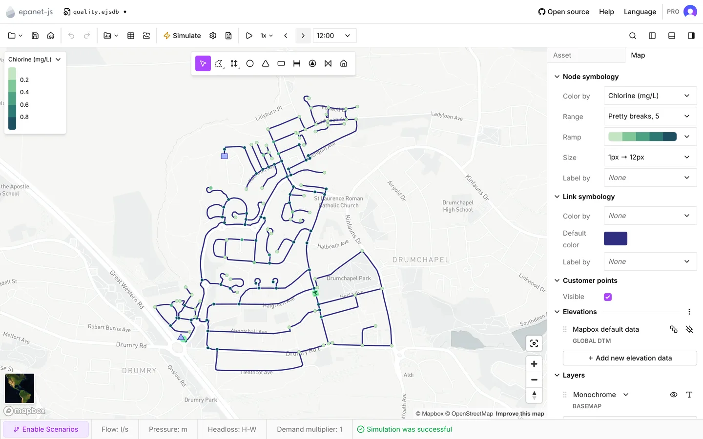
All of it follows the time browser. To watch a plume move or a tank turn over, color the map by the quality property and play the run back. See Reading results.
When you run a different analysis, the app clears anything set up for the old one. It does not leave stale numbers on show. A symbology colored by Water age loses its rule at your next trace run, and a quick graph goes back to the default property of its asset type.
The chemical name
Section titled “The chemical name”Chemical name is more than a caption for the report. When you type a name,
every row that would read Chemical is relabeled with that name, with a
capital first letter. This happens in the asset panel, the data tables, the
symbology list and both graphs. Type chlorine, and the network is colored by
Chlorine.
Mass unit is the odd row in the dialog. Its two choices are not a setting for the run. They are the concentration unit of the project. When you change it, the app relabels every concentration, and not only the ones that this run produced. See Simulation settings.
In a scenario
Section titled “In a scenario”As soon as one scenario exists, every row in the Water quality section becomes read-only, so that the engine solves every branch with the same analysis. The Quality rows on the assets stay editable, and that is what makes a scenario worth a run. You can move a source or change a coefficient on one branch, and compare the result against Main. To change the analysis itself, delete the scenarios. See Scenario work.
- Simulation settings — the rest of the dialog.
- Junctions, Tanks and Reservoirs — the rows each node carries.
- Symbology — coloring the network by the result.
- Graphs — the result over the whole run.