Customer points

A customer point is a property with a demand on it. It has a point on the map, a label, one or more demand categories, and a connection to a pipe. It is not an EPANET object. When you run the model, the app adds the demand of each customer point to the junction that the point is connected to. The engine sees ordinary junction demand. The customer points themselves are the record that epanet-js keeps of where that demand came from.

Customer points exist so that you can put a billing or property database into the model. Without them, you spread the demand over the junctions by hand. Both demo networks include customer points: Drumchapel has 1,171 and Waterdown has 2,010.

Three separate jobs put customer points into the model. They stay separate on purpose:

1. The import reads the points and their demands from a GIS file.
2. Allocation decides which pipe each point connects to.
3. Editing corrects the points that allocation got wrong.

Importing customer points

File > Import > Customer points opens the Import customer points wizard. The wizard is marked Early access, and you must be signed in to use it. If you are signed out, the entry opens the early access dialog first. See Accounts and privacy.

Caution

An import replaces every customer point in the project. If the model already has customer points, the app warns you first. The warning says that your current customer points will be permanently deleted and replaced with the points from your new import. Delete and import goes ahead with the import.

An import also clears more than the points. When the import finishes, it does three things:

• Resets the undo history.
• Discards the results of the last run.
• Puts the scenarios back to a single Main branch.

Save the project first. Do the import before you start scenario work, not during it. See Scenario work and Projects.

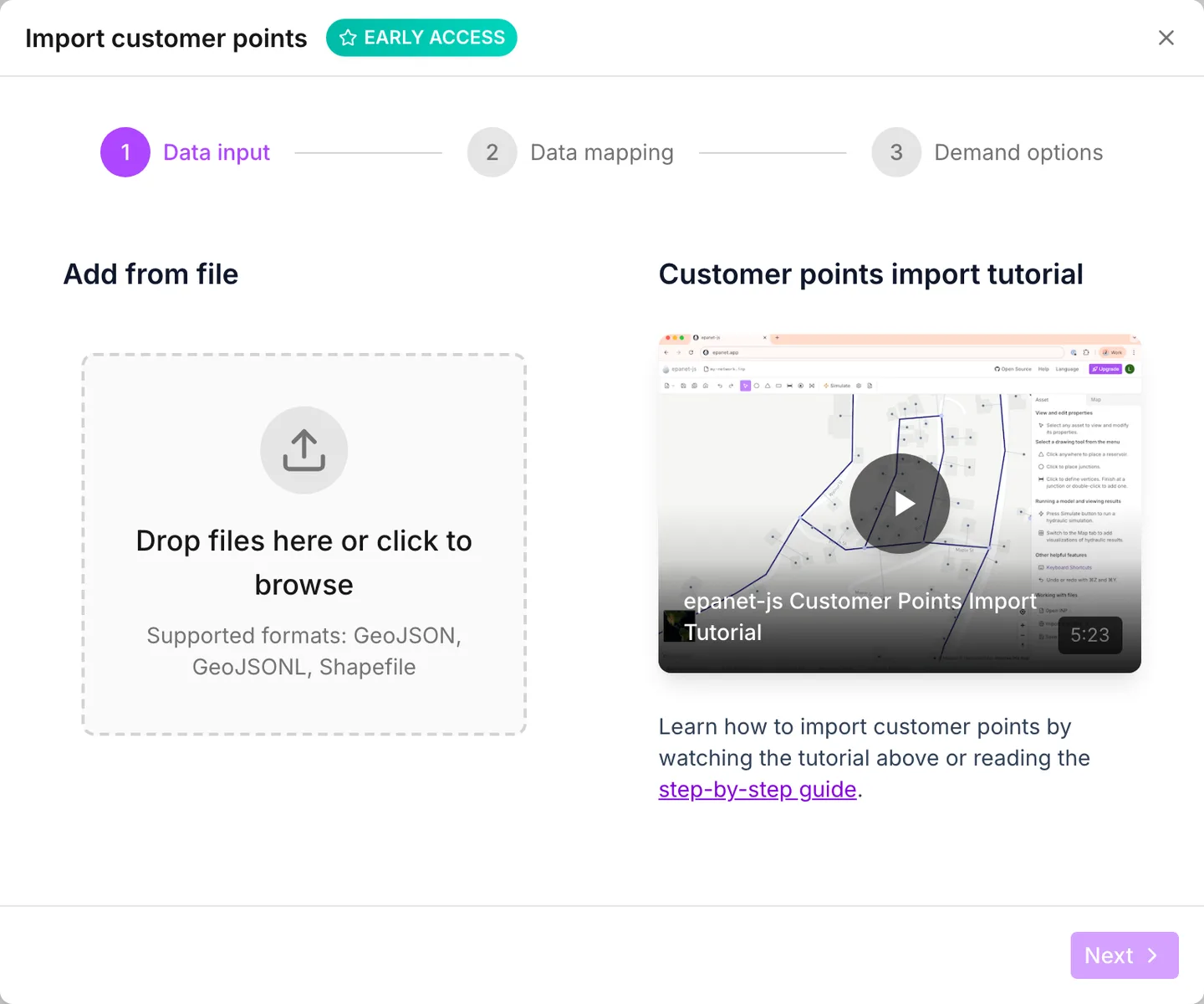
1. Data input. Drop a file, or choose one. The wizard reads GeoJSON, GeoJSON Lines (.geojsonl) and Shapefile. For a Shapefile, give the .shp together with its .dbf and its .prj. If the Shapefile has a .cpg, give that file too. Coordinates must be WGS 84, or the file must state its own coordinate reference system. The app converts a GeoJSON with a CRS definition, and a Shapefile with a .prj. It refuses a file that it cannot convert, with All coordinates must be expressed in WGS84 (EPSG:4326) projection, or include a CRS definition in the GeoJSON. When the file loads, the wizard moves to the next step by itself.

   

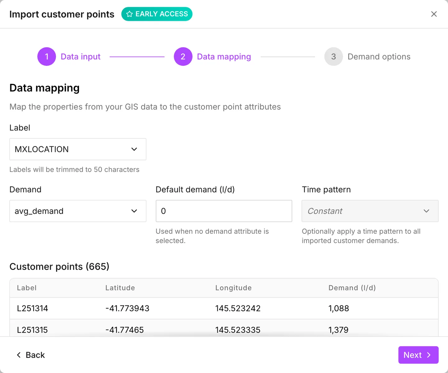
2. Data mapping. Tell the wizard which properties to read.

   • Label chooses the property that names each point. If you leave it on Auto-generate, the app numbers the points instead. A note under the selector says that labels are trimmed to 64 characters. The panel and the data tables use the same limit. See The Asset tab.
   • Demand chooses the property that holds the demand of each customer. The app reads this demand in the per-day unit of the project: l/d on a metric project, gal/d on a US one. This is the unit named beside Default demand, not the flow unit that the rest of the model uses.
   • Default demand is the demand that a point gets when you select no demand property. A point with a demand that the app cannot read also gets this value.
   • Time pattern applies one pattern to every imported demand. An empty Time pattern gives a constant demand. See Patterns.

   Under the selectors, Data preview lists the points as the app will import them, and an issues panel counts the rows with problems. The app skips a row in three cases:

   • The geometry is not a point.
   • The coordinates are missing or invalid.
   • The coordinates are not WGS 84.

   A skipped row is not imported, so the count in the table heading is what you get. The app also counts a row with a demand that it cannot read, but it does not skip that row. It imports the point with the Default demand instead. If no valid row is left, you cannot go on.

   

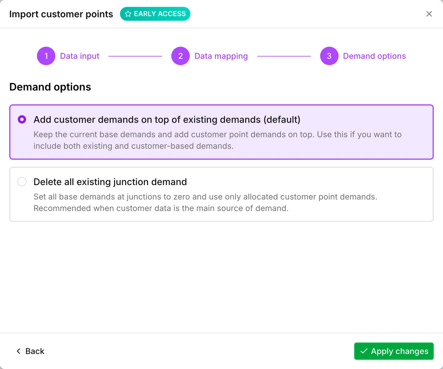
3. Demand options. Choose what happens to the demand already on the junctions.

   • Add customer demands on top of existing demands (default) keeps the junction demands as they are and adds the customer demand to them.
   • Delete all existing junction demand deletes every demand category from every junction. Then customer points are the only demand in the model.

   Apply changes finishes the import, and the app reports Import successful.

   

Every point arrives disconnected, because the import connects nothing. Allocation is the next step. Until you allocate the points, they add no demand to the run.

Allocating them to pipes

Allocate customer points is in the toolbar next to Save, and it opens Customers allocation. In a model with no customer points, it opens No customer points found instead. That dialog offers to do the import first.

Allocation connects a customer point to the nearest pipe that a rule allows. It then connects the point to the end of that pipe that is a junction. If both ends are junctions, it takes the nearer one. A candidate pipe must be enabled, must have a diameter, and must have at least one junction at its ends.

Note

Allocate customer points is unavailable in two cases: a project that has scenarios, and a project with no geographic projection. Allocation is a distance calculation, so a model with no projection has nothing to measure. See Projections.

Scope

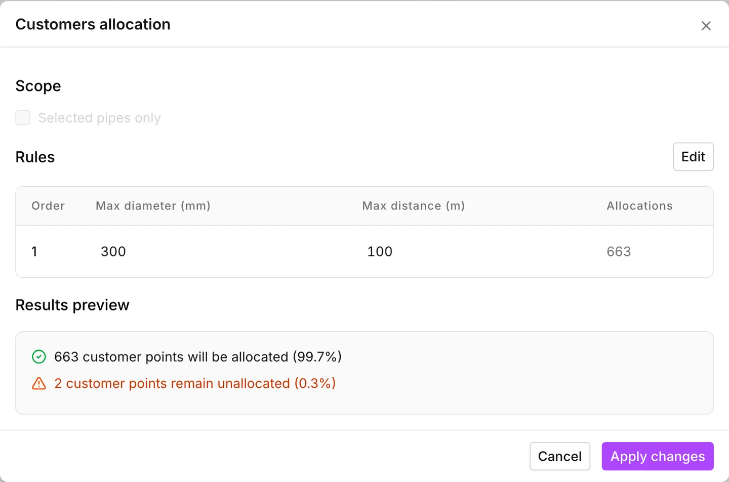
Scope, at the top of the dialog, narrows what the allocation covers.

• Allocation zone limits the allocation to the customer points inside the boundary of one zone. It appears only in a project that has zones, and its default is All zones. See Zones.
• Selected pipes only limits the allocation to the pipes you selected before you opened the dialog. If you selected no pipes, the tickbox is disabled.

A change to either one updates the preview.

Rules

Rules is an ordered table. Each row is a pair of values: Max diameter and Max distance, in the diameter and length units of the project. A row reads as “connect to a pipe no larger than this, and no further away than this”. A new project starts with one rule. That rule is 300 mm and 100 m on a metric project, and 12 in and 320 ft on a US one.

The order of the rows is important. The app tries each customer point against rule 1 first, then rule 2. The point takes the first rule that finds it a pipe. With this order you can say “connect to a service main within 30 m if there is one, and otherwise accept a trunk main within 100 m”. The tight rule goes first, and the fallback second. A single generous rule sends half of your customers to the trunk main.

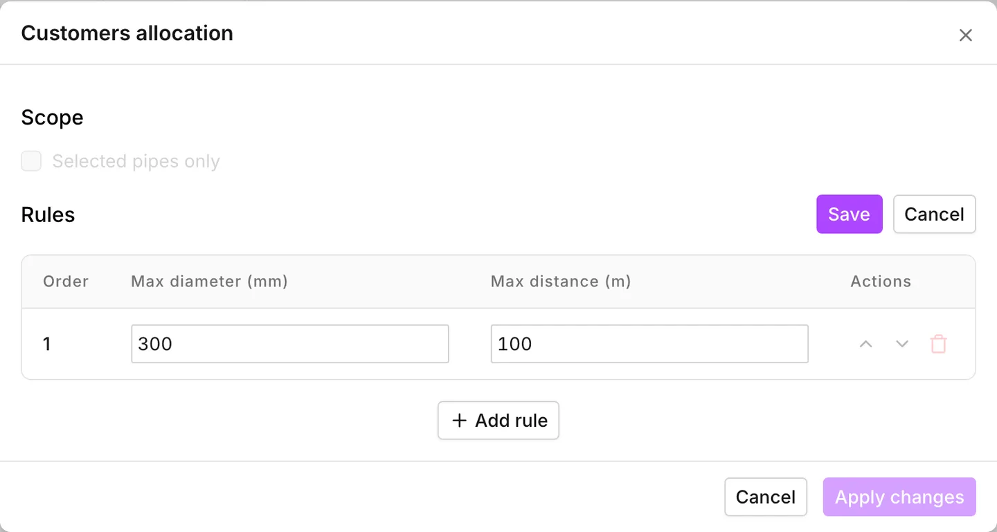
Edit unlocks the table. In the unlocked table you can do four things:

• Change either number in a row.
• Reorder the rows with Move up and Move down.
• Delete a row with Remove rule.
• Add a row with Add rule.

You cannot delete the last row. Save applies the edit and updates the preview. Cancel discards the edit. The app remembers saved rules, so the next allocation opens on the rules you used last.

Results preview

The Allocations column of the rules table shows how many points each rule caught. Under the table, Results preview gives the total: how many points the app will allocate, and how many it will leave over. Each number is a count and a percentage. In zone scope you get two totals: the coverage inside the zone, and the points that are still unallocated across the whole network.

Some pipes are excluded warns you that pipes in scope cannot take a customer, because they have no diameter or they are disabled. This warning is usually the reason a percentage is lower than you expected.

The model does not change yet. Apply changes commits the preview.

Caution

Allocation touches only the customer points that are disconnected. It leaves a point that already has a connection exactly as it is, whatever the rules say. If you change the rules and allocate again, nothing moves, and the summary reads No customer points to allocate in this scope. To allocate these points again, select them and Disconnect them first.

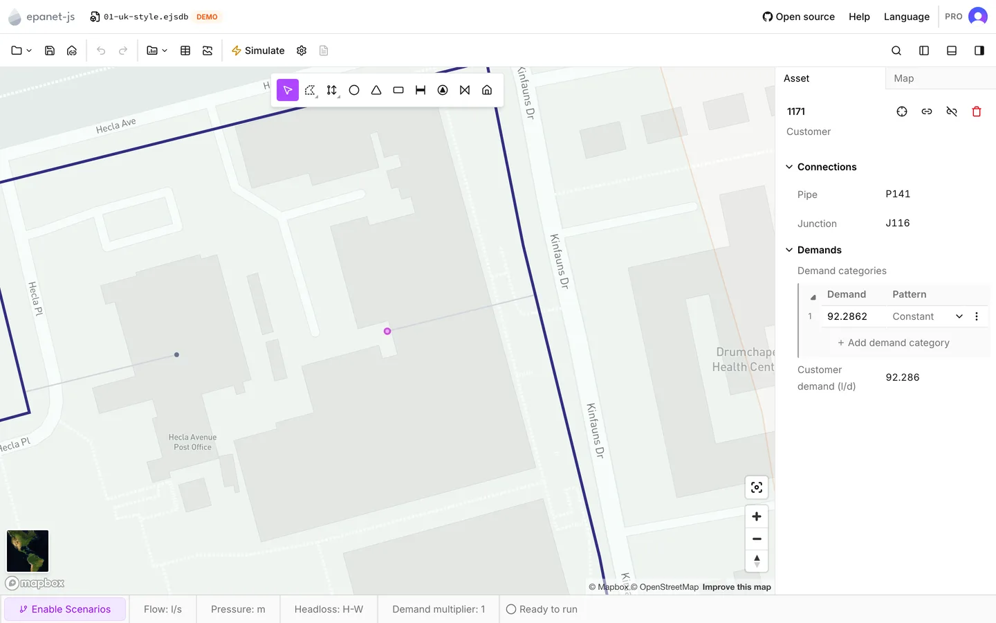
The customer point panel

When you select a single customer point, the side panel opens on the Asset tab, with Customer under the label. See The Asset tab for the panel itself.

The header carries Zoom to, then Connect, then Disconnect, and then Delete. On a point that already has a connection, Connect reads Reconnect. You can edit the label, but it must be unique among customer points. The app refuses a label that is in use, with Label already in use.

Connections appears only on a connected point. It has two read-only rows: the Pipe that the point is connected to, and the Junction that its demand is applied at.

Demands holds a Demand categories grid with a Demand column and a Pattern column. It is the same grid that a junction has. Under the grid, a read-only Customer demand row gives the pattern-weighted average. On a point with no demand yet, the section shows only Add direct demand. Every value here is in the per-day unit, not in the flow unit of the project.

Custom attributes appears when the project defines custom attributes for customer points. See Custom attributes.

Connecting and disconnecting

Connect or Shift+C puts the map into a connect mode: Click on a pipe to connect the customer point. Move the cursor near a pipe, and the app shows where the connection will land. Click to make the connection.

Shift decides where the connector lands. Without this key, the connection goes to the nearest point on the pipe, which is the perpendicular. With it, the connection goes to the cursor. Use it to put a service connection at a particular spot along the main. If you leave the mode with Esc, nothing is connected.

Disconnect or Shift+D breaks the connection. The point stays on the map with its demand intact, but it adds nothing to the run, and Network Review reports it. You can disconnect a whole selection. When a multi-selection holds customer points, the Asset tab header offers Disconnect customers. See Selection and search.

Two actions disconnect points without a request from you. When you delete a pipe, the app disconnects the customer points that the pipe carried, and does not delete them. When you split a pipe, the app reconnects them to the half that is now nearer. See Drawing and editing.

On the map

The map draws customer points as small dots. A thin line goes from each dot to the point on the pipe that it is connected to. A disconnected point is a dot on its own.

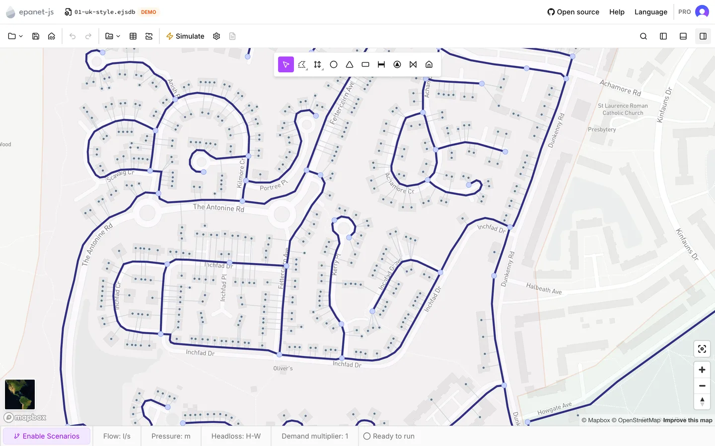
• The map draws them only at zoom 14 and closer. Further out, the map shows none of them, and Ctrl+A selects none of them.
• Customer points > Visible in the Map tab turns them off completely. It also takes them out of the current selection. See Symbology.
• The map draws a point connected to a disabled pipe in gray, and its demand does not reach the run.
• The Customer point tool, 8, places a point where you click. The new point has no demand and no connection, and the app selects it for you. See Drawing and editing.
• Select a point and drag it to move it. The connection does not follow. The point keeps the same pipe and the same point on that pipe, so the connector line gets longer. If the connection must move too, press Reconnect after the drag.

Where customers appear elsewhere

• On a junction, Customer demand, Customer demand pattern and Connected customers appear when points are connected to its pipes. Connected customers is a count. Click it for the list, which highlights those points on the map. See Junctions.
• On a pipe, the same three rows appear under Demands. They count the points connected to that pipe. See Pipes.
• When you select several points, the multi-asset panel gives a Customer points section. It shows Connected across the selection, with their Number of demands, Customer demand pattern and Customer demand. See The Asset tab.
• The Customer points tab of the data tables has one row per point. The row holds Label, the read-only Pipe and Junction, a read-only Customer demand and Number of demands, and an editable Base demand and Pattern. While customer points are hidden, Select in map on a row does nothing.

What reaches the run

For each enabled junction, the model adds the demand of every customer point connected to that junction, grouped by pattern. It writes one demand line per pattern, beside the demand categories of the junction. A customer point with a demand of zero is left out, and so is a point on a disabled pipe.

An exported INP carries that aggregated demand, because the app writes it as ordinary junction demand. But the INP does not carry the customer points themselves. Only an epanet-js project file (.ejsdb) keeps the points, their labels, their own demands and their connections. See Import and export and Projects.

Network review reports a disconnected customer point as Customer point disconnected, which is a warning. Warnings block the pre-run check in the same way as errors. A model that you imported but did not allocate stops at the dialog before Simulate.

Next

• Junctions — where customer demand ends up.
• Zones — the polygons an allocation can be confined to.
• Patterns — the profiles an imported demand can carry.
• Network review — the disconnected-customer warning.