Build a model from GIS

This is the first of the three jobs people arrive with. You have GIS layers of the network, and no hydraulic model. The layers are pipes, and usually some point layers for valves, pumps, tanks and reservoirs. The model builder takes those layers, works out the topology from the geometry, and gives back an epanet-js project you can run.

If instead you already have an INP or a project file, go to Open an existing model. If you have a model and want to test changes against it, go to Scenario work.

A recorded walkthrough shows the whole job on real utility data: GIS to EPANET tutorial: Building the Rosebery water model with epanet-js. It runs about 25 minutes. The written version of the same build is Worked example: Rosebery.

What you need

You must be signed in on the Pro or Teams plan, or be in a free trial. The window must also be at least 768 px wide. Then two entries open the builder directly: Import from GIS on the welcome dialog, and File > New project > From GIS data. A narrower window shows neither entry.

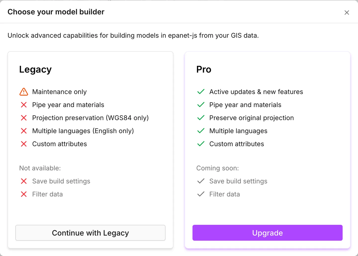
On any other plan, the same entries open Choose your model builder first. That dialog offers Upgrade on one side and Continue with Legacy on the other. A guest is treated as a free plan. See Plans.

The legacy builder is not this page

Continue with Legacy opens a different app, the one that the builder replaced. That dialog marks it Maintenance only, and lists what it costs you: no Pipe year and materials, WGS 84 output rather than your own projection, English only, and no Custom attributes. If you get to it while signed out, Early access feature and Get early access appear first. This page does not describe that app. Every step, every label and every frame here is the builder that the Pro and Teams plans open.

Your layers must be GeoJSON, Shapefile, DXF or CSV files. The dropzone reads Supports GeoJSON, DXF, CSV, Shapefiles, and ZIP archives. You can drop a Shapefile as its loose parts. The builder groups the .shp, .dbf, .prj and .cpg files into one entry. An entry that has no .shp file yet waits, and shows Add the .shp file.

A .zip can hold either kind, or a whole folder of layers. The builder expands archives in the browser. It flattens folders to their file names, and it reads one level of nested zip. If two layers in different folders have the same file name, they collide. Rename one of them before you zip them.

The builder puts files of a kind that it does not read into one summary, Files not supported. Show ignored files lists them. If a file of a supported kind does not load, the builder reports it under Couldn’t load 2 files. A corrupted .zip is one such file. The report gives the name of each file and the reason, for example Unreadable or corrupted file or No records with valid geometries found. A Shapefile that does not load is different. It stays on the list, with the reason on its entry.

A CSV holds points, with their coordinates in two of its columns. The builder does not guess which two, so the file asks you to Select the attributes holding the coordinates. Choose them in X / longitude and Y / latitude. Then the points appear on the preview map, and the file reads Check the map, then confirm the attributes. The tick beside the two selectors, Apply attributes, confirms them.

A CSV cannot state a coordinate system. Thus, if the coordinates are not longitude and latitude, the builder asks for a projection. It does the same for every other file that does not name one. You can choose the columns again with Change coordinate attributes, in the file’s menu.

The first row must name the columns. If a CSV has no header row, the builder does not load it, and reports No header row naming the columns. If a CSV has fewer than two numeric columns, the builder reports No attribute holds coordinates.

Note

The builder starts a blank project first. If the project you have open has unsaved changes, Unsaved changes appears before the builder. It offers Save and continue and Discard changes.

What the builder works out for itself

Most of the preparation people expect to do by hand is unnecessary here. Knowing which parts are unnecessary is most of the work of a clean build.

• Connectivity is derived, not read. There are no from-node and to-node fields to map. The builder creates a node at each end of every pipe, and at every point in the network layers you assign. A customer point is not a node, and a zone is not part of the network at all. The builder merges points within about 0.1 m of one another into a single node. That tolerance is the one number to know before you start. For two pipe ends to connect, they must coincide in the data. A gap wider than 0.1 m leaves two nodes and a break in the network.
• Points split pipes. A point that lies on a pipe splits it. A tank, reservoir, valve or pump digitized on a main becomes a node on that main. The builder splits the pipe on each side of that node.
• Valves and pumps become links. EPANET needs a valve or a pump to be a link between two nodes. Your data has them as points. The builder converts each one into a short link, and shortens the pipe it sits on to make room. These are the Converting nodes to links and Expanding short links stages of the build.
• Lengths are measured, not mapped. Pipe length comes from the geometry, in meters or in feet according to the flow units you chose. The builder deletes pipes that have no length, at Removing zero-length pipes.
• Elevations are fetched. If the geometry carries a Z value, the builder uses it. Otherwise the builder reads node elevations from a terrain service, at Getting elevations. If the service has no answer for a node, the builder leaves that node without an elevation, not zero, because zero is sea level. The build warns you with a count of these nodes. See Elevations for how to compute them again afterwards.
• Nothing unmapped is invented. The builder imports an attribute you leave unmapped as empty, except for the few rows whose selector reads Use default value. An unmapped reservoir Head, tank level or diameter arrives blank, not as a placeholder. After the model opens, the Model attributes check in Network review reports the blanks.
• Identifiers come from your data or from the builder. If your data has an identifier, you can map that property to ID. The builder then makes duplicates unique with a suffix. If you leave the row on Auto-generate, the builder numbers by type instead: J1, J2 for junctions, and R, T, P, V and PU for reservoirs, tanks, pipes, valves and pumps. Your choice becomes the label of the asset in the app.

Projection

The builder reads the projection from the data, file by file. It reads the .prj of a Shapefile, the CRS that a GeoJSON declares, or the coordinate system that a DXF declares. A file in latitude and longitude needs nothing, even when you drop it together with projected layers. The builder reprojects each file on its own, or leaves it as it is. Thus a WGS 84 layer can go into the build unchanged.

If the builder cannot identify the coordinate system of a projected file, that file waits for you to choose one. It reads Select its projection. A Shapefile with no .prj reads Add a .prj or select a projection. The other files do not wait.

Search by name or by code in Projection name or EPSG…. Before you type, the list suggests the projections that the other files in the build already use. After you choose one, the records of the file appear on the preview map. The file then reads Check the map, then confirm the projection. The tick beside the search, Apply projection, confirms it.

If a projection does not fit the coordinates, the file reads Projection doesn’t match. Select another. This is true for a projection that you chose and for one that the file stated. Then you choose again. If a file states a projection that the builder does not support, the file reads Unsupported projection. Select another.

The project takes its projection from the pipe layer. If there is no pipe layer, the project takes its projection from the first of the junction, valve, pump, tank and reservoir layers that you assign. The model then opens in the app in the coordinate system of that layer. See Projections.

The four steps

Buttons at the foot of each step move you between the steps. Each button has the name of the step that it leads to. File upload leads on from the settings, and Attribute mapping leads on from the files. Intro and File upload lead back.

The frames that follow come from one real build: the watermains, tank and water treatment works of Rosebery, in Tasmania. That build is written up in full as Worked example: Rosebery.

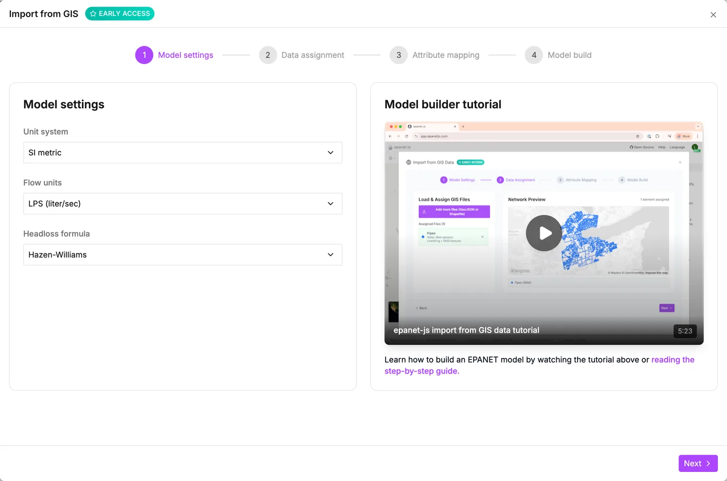
1. Model settings

   Unit system switches between US customary and SI metric. Your choice sets the list that Flow units offers. Headloss formula chooses between Hazen-Williams, Darcy-Weisbach and Chezy-Manning.

   These settings decide the units of every later step, including the units that your diameters and levels are assumed to be in. Set them before you load anything. The panel beside them holds the Model builder tutorial video.

   

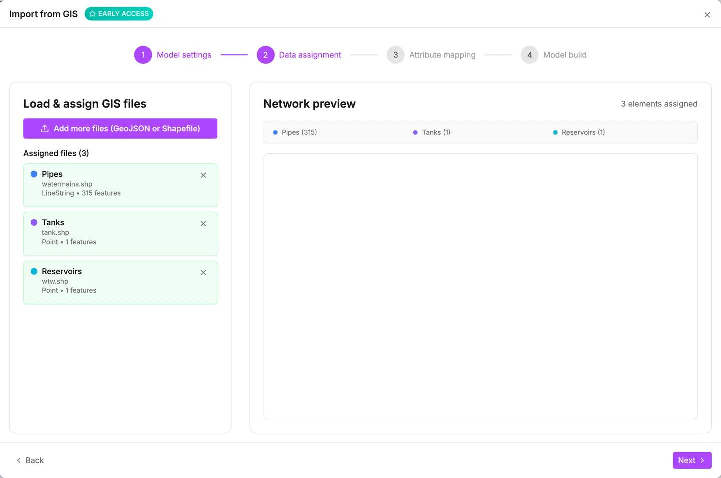
2. File upload

   Drop your files. They go into a list, Data sources. Add data source adds more files. A mark beside each name shows the state of the file: ready, needs attention, failed, or still loading. A file that needs something says what under its name. First it gives its geometry and record count, as in Lines – 315 records. Then it gives the part or the projection that it waits for.

   Assign each ready file to an element with Assign to element…. The eight elements are Pipes, Junctions, Valves, Pumps, Tanks, Reservoirs, Customer points and Zones. Pipes take line geometry, zones take polygons, and the other six take points. If the geometry of a file does not fit an element, the builder does not offer that element for the file. If the builder cannot identify the geometry of a file, the file reads Unsupported geometry. The builder offers no element for it.

   If a file holds more than one kind of geometry, the builder splits it by geometry. You assign each part on its own, with Assign points to, Assign lines to and Assign polygons to. Thus one file can give the pipes and the valves. Each element takes exactly one layer. After an element has a layer, the builder does not offer it again. A layer that has no element left to go to reads No compatible elements left.

   Unassign, in the file’s menu, frees the elements of the file again. The file stays on the list, unchanged. Remove source takes the file off the list.

   The pipe layer is the one the build works from, and it is the only one the builder truly needs. Junctions are created at pipe ends, with or without a junction layer. Assign a junction layer when your junction attributes matter, or when there are nodes that no pipe end lands on.

   Customer points and zones go into the build with the network, but they are not part of the network. A customer layer is the same service-point file that Customer points imports. A zone layer is the same polygons that Zones imports. If you assign them here, the two imports are not necessary afterwards. But customer points and zones alone do not let you continue. Attribute mapping stays disabled until you assign at least one network layer.

   If you leave a ready file, or a part of one, unassigned, the builder leaves it out of the model. Before you move on, the footer tells you: No element type is assigned to hydrants, so they won’t be included in the model. Continue anyway moves on without it. Keep editing stays on the step.

   

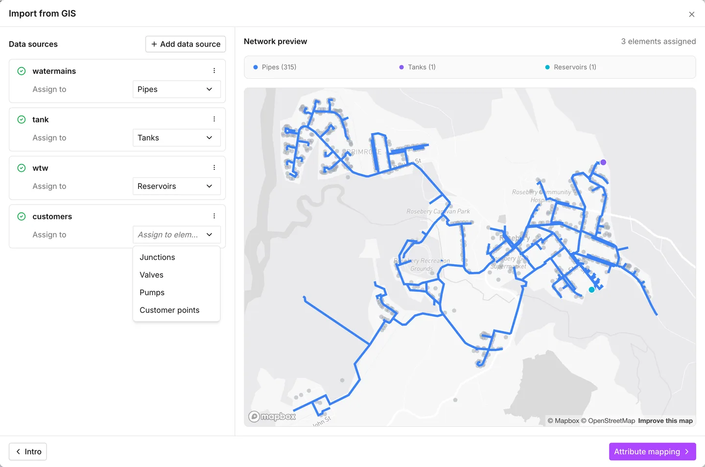
   Network preview shows what you assign, while you work. If a projection is wrong, you see it at once: the network is in the wrong place, or at the wrong scale. Change projection, in the file’s menu, unassigns that file and asks for its projection again. If a file has more than 50,000 records, the preview shows only a sample, and tells you: The preview draws a sample of the records. Every one is still imported. The sample applies to the map only, not to the build. Every record in that file goes into the model.

   

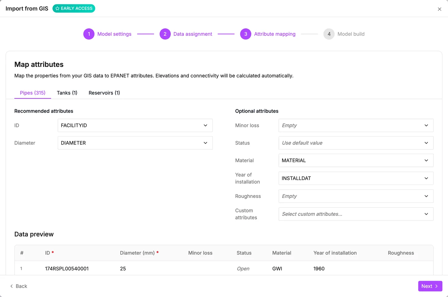
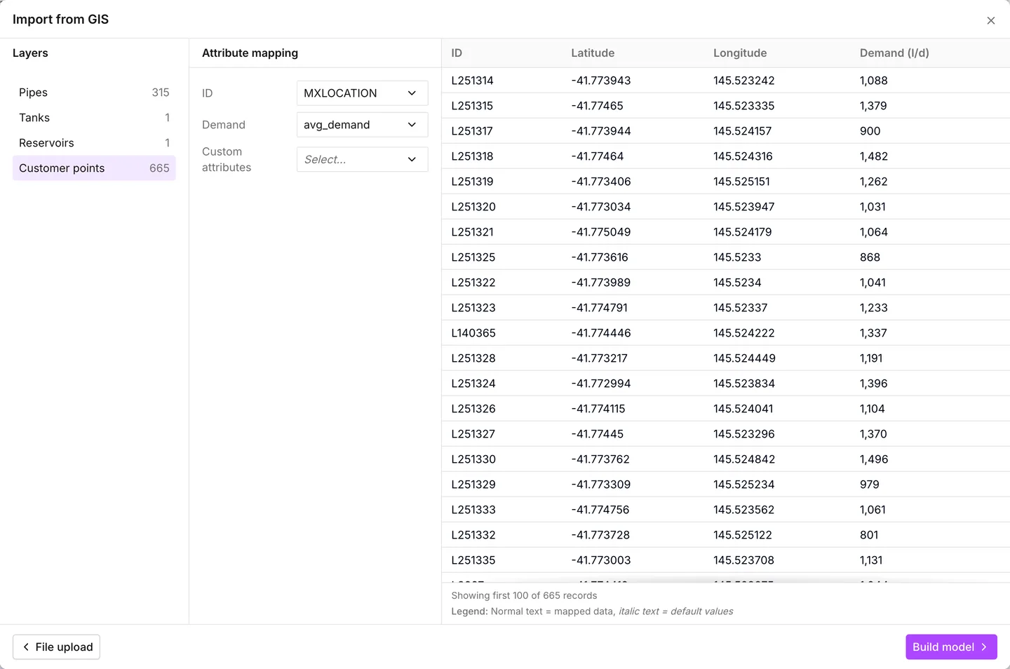
3. Attribute mapping

   Layers, down the side of the step, lists each assigned element with the record count beside its name. Click an element in this list. Its rows then appear in the Attribute mapping column beside the list. A preview of its records appears beside that column. For each row, choose the property in your data that holds that attribute.

   

   The rows differ by element:

   • Pipes have ID, Diameter, Minor loss, Status, Material, Year of installation and Roughness.
   • Valves have ID, Diameter, Type, Setting, Minor loss and Status.
   • Tanks have ID, Initial level, Min level, Max level, Diameter and Min volume.
   • Junctions have only ID. Pumps add Status, and reservoirs add Head.
   • Customer points have ID and Demand. The builder reads the demand in the per-day unit of the project. The preview names that unit in the header of its Demand column: liters a day on a metric project, gallons a day on a US one. A point with no demand property arrives with no demand. The preview for this layer has its own columns: ID, Latitude, Longitude and Demand. These coordinates are in longitude and latitude, whatever the projection of the source file.

   

   • Zones have only ID. Records that share a label become one zone. The preview lists the zones, each with its label and its number of Polygons. Auto-generated labels never merge. The builder numbers these zones Z1, Z2 and so on.

   

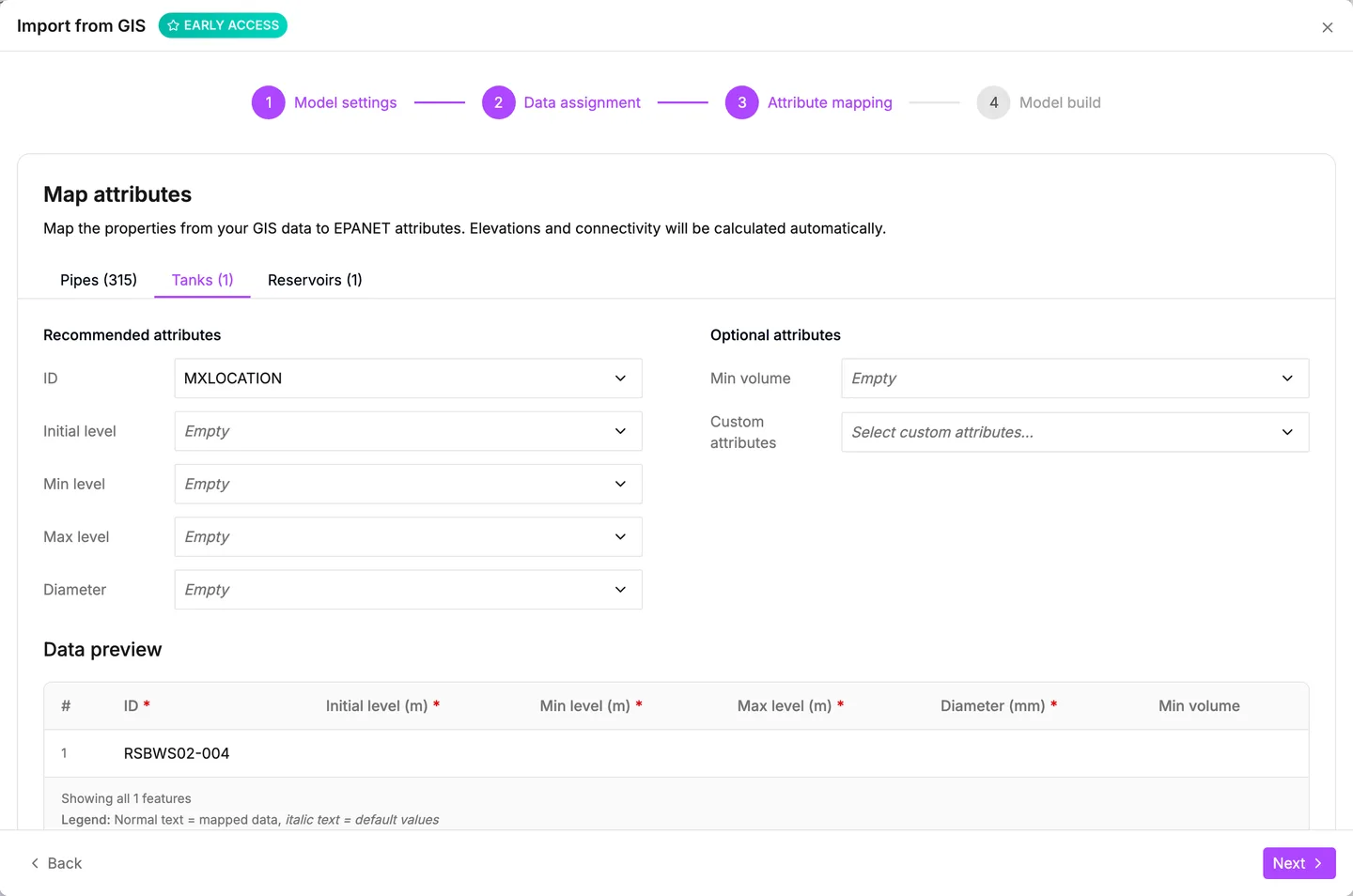
   If you leave a row unmapped, that is also a decision, and the selector shows which decision it is. On an ID, it reads Auto-generate. Where the builder has a default for the row, it reads Use default value. Where the builder has no default, it reads Empty, as on pipe Roughness. A row offers the list of columns in that layer, not the values in them. The values are in the preview, beside the mapping.

   

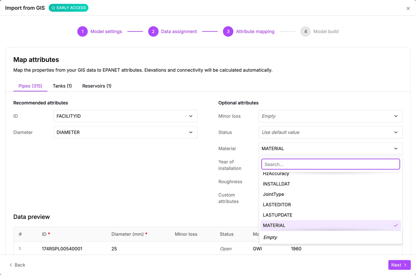
   Custom attributes is under the rows of the network layers and of customer points. It takes as many more properties as you want, and carries them into the model unchanged. This is how a material class, an asset reference or a survey date survives the build. See Custom attributes.

   The preview shows the first 100 records as the builder will import them. Values that come from a default are in italics. The footer of the preview counts the records, as in Showing first 100 of 315 records. The preview also shows bad values. If the builder cannot read a year, a status, a valve type or a valve setting, the preview flags that value. It also shows the value that the builder will import instead.

   Fix those values in the source data, or map a different property. Do not leave them for later.

   Build model, at the foot of the step, starts the build. If a layer has nothing mapped, not even a custom attribute, the builder uses only default values for it. In that case, the footer tells you first: No attributes are mapped for Valves, so they will be built with default values. Build anyway starts the build. Keep editing stays on the step.

4. Model build

   Building EPANET model lists each stage when it finishes, with its duration. Nothing here needs an answer from you. Read the warnings. An elevation warning gives the number of nodes that got no elevation, and the reason. Either the builder could not connect to the terrain service, or the service has no data for that area.

   A customer layer adds an Importing customer points stage after the elevations. A zone layer adds an Importing zones stage. If a stage skips records, it warns you, as in these two messages:

   • 12 of 665 customer points were skipped. Check they have point geometry and a valid projection.
   • 2 of 11 zone records were skipped. Check they have polygon geometry and a valid projection.

   The builder imports the rest of the file. If the geometry of a record is not the kind that the element takes, the builder skips that record. It also skips a record whose coordinates did not survive the projection.

   A build that warns waits for you, and does not close over the message. After you read the warning, press Open model. A build that does not warn hands the model to the app by itself.

   

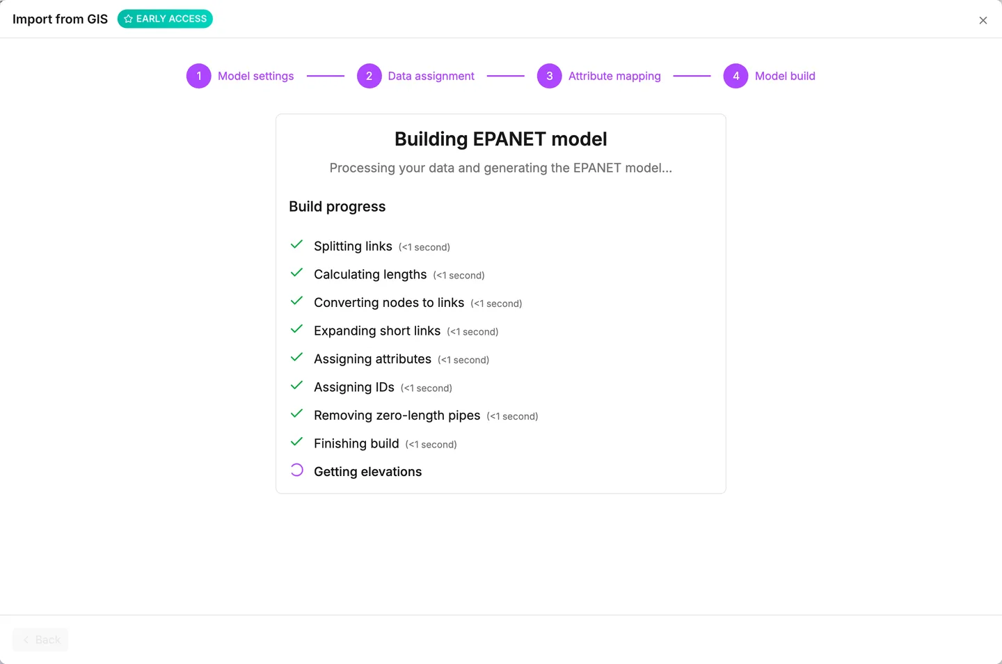
   A build that fails ends on Build error with the message, and Show more expands it. Back returns to the mapping, with everything you set still in place.

What you get

The model opens in the app as an unsaved project, named after the build. Network Review opens beside it on its own, because a new model is where its checks matter most. Orphan assets and Connectivity trace show where the 0.1 m tolerance left real breaks in the network. If the build included customer points, the review also reports every one of them as Customer point disconnected. The builder places the points but connects none of them. Allocation is the next job.

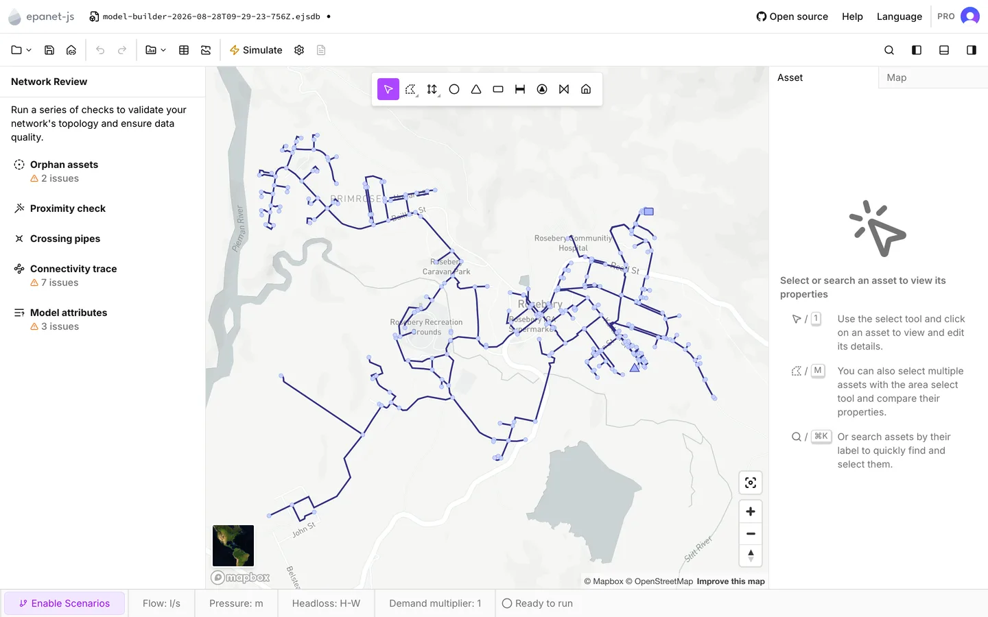
Save the model before anything else. Save writes an .ejsdb project file to a location you choose. Until then, the model exists only in the browser. See Projects.

Then add the operational data that the GIS did not have. A built model arrives with geometry, connectivity, elevations and the attributes you mapped, plus the customer points and zones you assigned, and nothing else. There is no junction demand, no pump curve, no pattern and no control. A customer point carries its demand, but adds nothing to a run until you connect it to a pipe. The simulation duration is zero, which is a single-period run.

• Demands, one junction at a time or in bulk — see Junctions and demands and Data tables. Customer points give demands too. Allocate them to pipes with Allocate customer points — see Customer points.
• Pump duty points — see Pumps and Curves.
• Patterns and Controls. Then set a duration in Simulation settings to make it an extended-period run.
• When the review is clean, press Simulate. See Running a simulation.

Next

• Network review — the five checks, and which ones block a run.
• The interface — where everything is in the window you now see.
• Drawing and editing — how to fix the breaks the review finds.
• Projections — how to change the projection after the build.
• Plans — what the Pro and Teams plans include.