
Worked example: Rosebery, TAS
Rosebery is a small mining town on the west coast of Tasmania. Its water is treated at works below the town. The water is then pumped up to a service reservoir on the hill, and it gravitates back down through about 20 km of main. This page builds that model from the utility’s own GIS extract, and takes it as far as a controlled 24-hour run.
The work divides in two, and the second half is the longer one. The GIS import takes four screens. The rest of the page turns what arrives into something EPANET can solve. That work joins a network the extract left in pieces, and adds a pump that was never in the data. It also gives the tank a shape, gives the pipes a roughness, and puts demands on the model from a customer layer. This second half is the part that transfers to your own data.
This same build is on video, in GIS to EPANET tutorial: Building the Rosebery water model with epanet-js. The recording is about 25 minutes long, and this page follows it.
This page is the counterpart to Draw a model, which draws a network from nothing. Here you draw almost nothing, because the work is in the data.
What you need
Section titled “What you need”You need the sample data: Rosebery GIS files (105 KB). Unzip the file somewhere you can drag files from. It holds four layers:
| File | What it is |
|---|---|
watermains.shp and its sidecars |
315 mains, with FACILITYID, DIAMETER, MATERIAL and INSTALLDAT |
tank.shp and its sidecars |
the service reservoir, one point, with MXLOCATION |
wtw.shp and its sidecars |
the treatment works, one point, with MXLOCATION |
customers.geojson |
665 metered connections, with MXLOCATION and avg_demand |
All four layers are in GDA94 / MGA zone 55, and each one carries its own
projection. The Shapefiles carry it in a .prj file, and the GeoJSON carries it
in a crs member. It is not necessary to reproject anything first. See
Projections.
One change was made to this extract before it got here, and it is a good change to make to your own. Assets that the utility abandoned were filtered out. Nothing in the model builder can tell a decommissioned main from a live one.
You also need an account. The GIS import is on the Pro and Teams plans. The customer point import needs you signed in. The pipe library and the pump’s native controls are paid features, and Part 5 gives a route around the native controls. See Plans.
Part 1 — Build the network
Section titled “Part 1 — Build the network”Choose Import from GIS on the welcome dialog, or File > New project > From GIS data. Build a model from GIS describes the builder in full. This part covers only what to do with these three layers. The customer file is not one of them, because it comes in later, through the app.
-
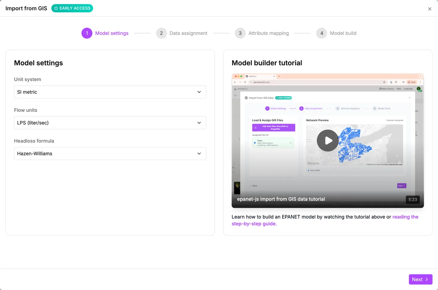
On Model settings, set Unit system to SI metric. Flow units then reads Liters per second (LPS), and Headloss formula reads Hazen-Williams. This build wants those two values, so change nothing else on the screen.
-
Press File upload. Drag in every file for each layer, not only the
.shp. The app groups the.shp,.dbf,.prjand.cpgfiles of one layer into one entry. If an entry still has no.shp, the entry says so. Then assignwatermainsto Pipes,tankto Tanks andwtwto Reservoirs.Network preview draws each layer as you assign it. Use the preview to make sure that the projections were read. A
.prjfile that came through correctly puts Rosebery in Tasmania, not in the Gulf of Guinea.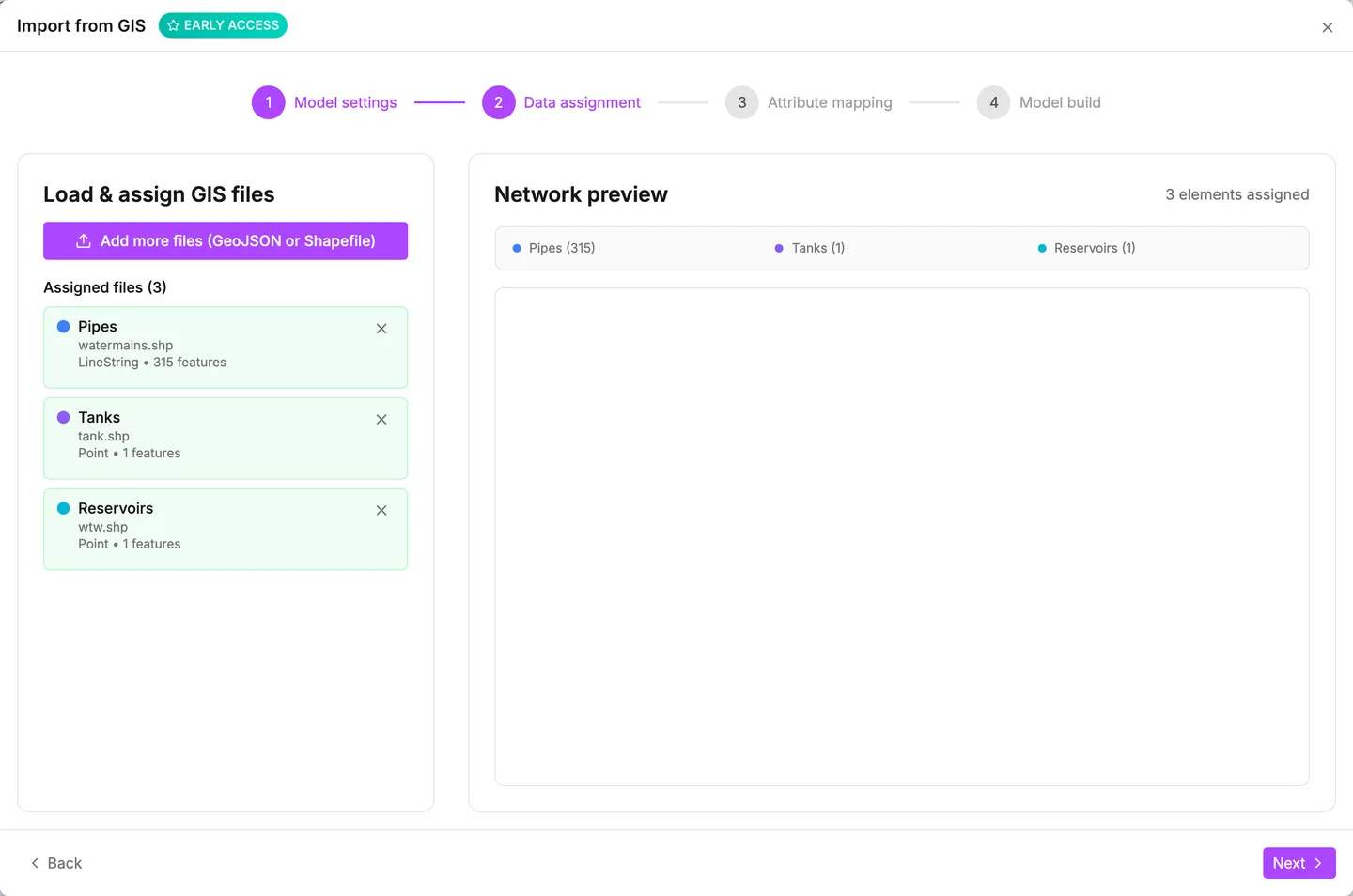
-
Press Attribute mapping. Layers lists the three layers. On Pipes, map ID to
FACILITYID, Diameter toDIAMETER, Material toMATERIALand Year of installation toINSTALLDAT.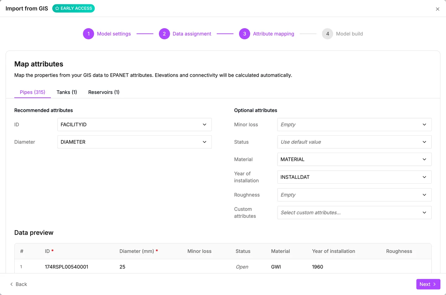
Each selector lists every column in the layer. A search box above the list helps when an extract carries many columns.
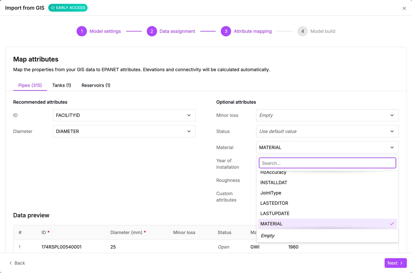
The preview beside the mapping shows the first rows as the builder reads them. Before you build the network, use the preview to make sure that a column holds what its name suggests. Values in italic are the default values that the builder uses where no column is mapped.
Roughness stays unmapped, because the extract has none. That is deliberate, and the middle of this page solves the problem.
-
On Tanks and Reservoirs, map ID to
MXLOCATION, not to theFACILITYIDthat the pipes used. The point layers carry their operational name inMXLOCATION. The tank keeps that name,RSBWS02-004, for the rest of this build.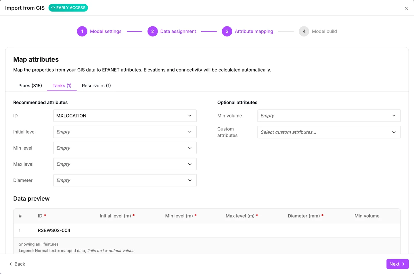
-
Press Build model. The builder reports each stage as it works. It connects the pipes at every intersection, applies your attributes, and reads the elevations off a global terrain model. It then turns the point layers into a tank and a reservoir.
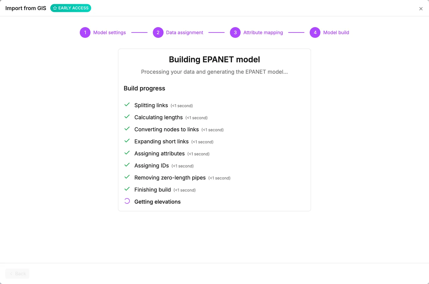
What comes back is 338 junctions and 348 pipes. Every pipe has a material and no pipe has a roughness. The tank is at 237.3 m and the reservoir is at 162.7 m. The model will not run yet, and there is no point in pressing Simulate to find that out.
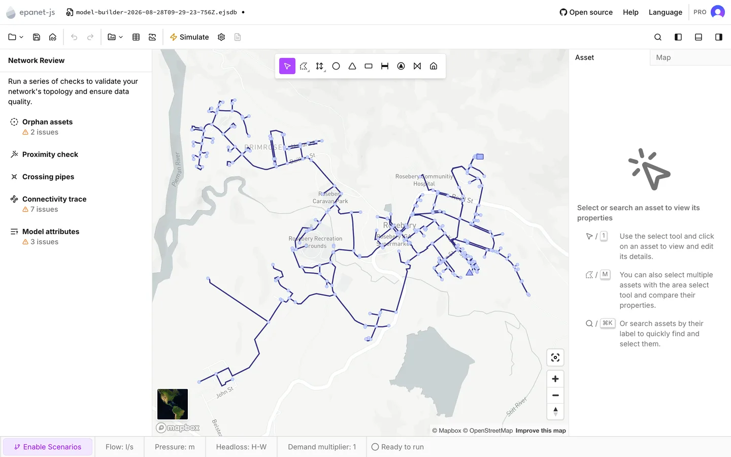
Part 2 — Make it run
Section titled “Part 2 — Make it run”Press Simulate anyway, once, to see what stops the run. The three blocking checks run first, and the run halts at Before running the simulation. That dialog names up to three of the failing rules and counts the rest.
Two rules stop the run here. Parts of the network connect to no source of supply. The attributes that the extract never carried are also missing: the tank’s levels and shape, the reservoir’s head, and a roughness on every pipe. The builder invents none of them, so what the data did not have, the model does not have.
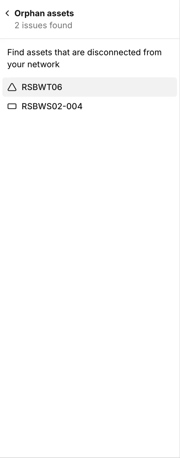
The tank and the reservoir are attached to nothing as well, and Orphan assets lists both. An orphan tank or reservoir is the one finding that does not block a run. Review issues takes you to the panel. Run anyway hands the model to EPANET, which reports the same things in its own terms and less usefully.
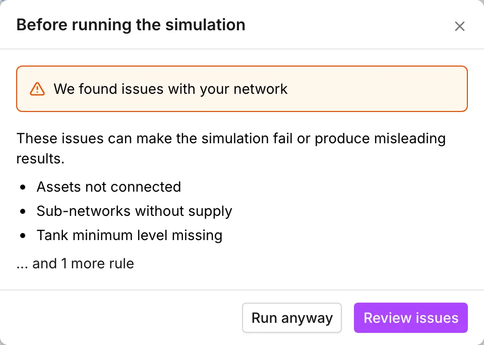
Press Review issues. The Network Review panel also opens by itself after a build. Toggle left panel at the right of the toolbar opens the panel again at any time. Ctrl+B also opens it.
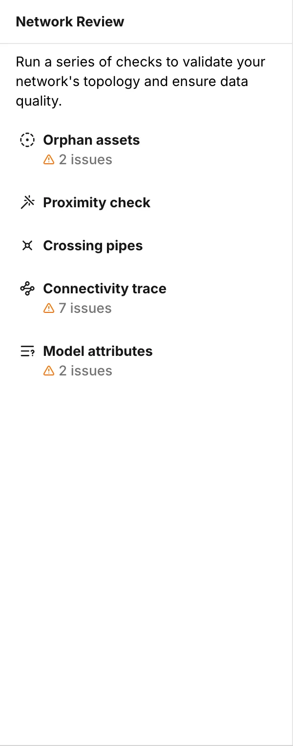
The panel lists five checks. This build works through them in a different order from the panel, and it starts with connectivity. Until the network is one piece, the other checks report on a shape that is about to change. Network review covers all five in detail.
Connectivity trace
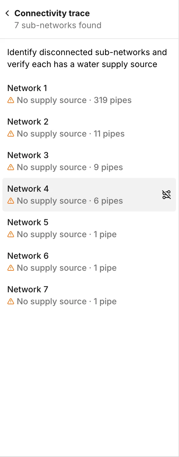
Section titled “Connectivity trace”Connectivity trace splits the model into sub-networks and marks the ones with no source. A GIS extract of a small town is normally one network and a few strays. Rosebery comes in as several sub-networks, and seven of them have no supply.
When you select a row, the app selects every asset in that sub-network and zooms to fit it. The map tells you what the sub-network is faster than any attribute does.
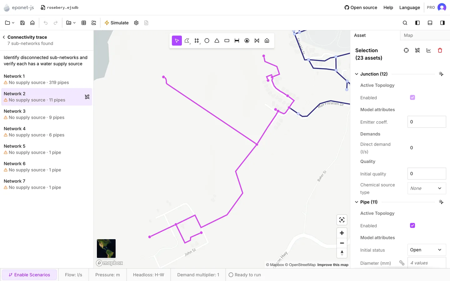
They come in three kinds here, and each has its own answer:
- A real gap. Two parts of the distribution network meet at a point where the digitizing left two nodes that look coincident but are not the same node. Zoom in until you can see both, then drag one onto the other. They merge into a single node.
- Drainage in the mains layer. A run of pipe by the tank is not potable main at all. Select it and delete it.
- The rising main. The line from the treatment works to the tank comes in as its own sub-network, disconnected at both ends. Merge a node at each end, in the same way.
The direction of the drag matters, because a merge keeps the position of the node you drop onto. Drag the loose end onto the node that is in the correct position, never the other way round. See Drawing and editing.
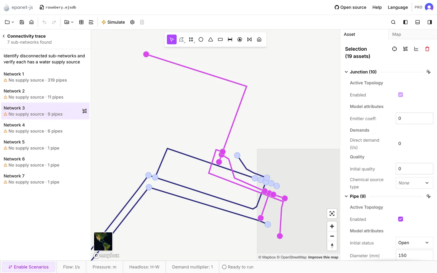
Three more stray fragments are left after that. They are odd private lengths that the extract picked up. Delete them. You are finished when the check reports one network with a supply source.
Orphan assets
Section titled “Orphan assets”Orphan assets starts at two, the tank and the reservoir. Each one is a single point in its own layer, and nothing in the data says which main it belongs to. The connectivity work corrects both, because the merge at each end of the rising main is what attaches them. When you come back to this check, you can expect it to be empty.
The pump
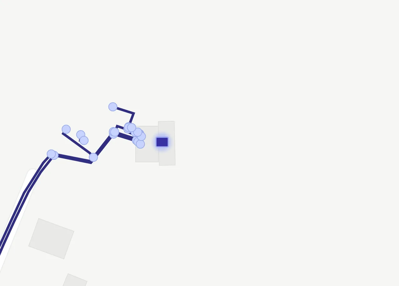
Section titled “The pump”There is no pump in the GIS, and without one the reservoir at 162.7 m cannot fill a tank at 237.3 m. Add the pump at this point, while the rising main is in front of you.
Take the Pump tool from the map toolbar (key 6). Hold the pointer over the
rising main where the pump belongs, just above the treatment works. The pipe
highlights at the point where the pump goes in. Click there. The app cuts the
pipe and puts the pump between the two halves, so the pump replaces a stretch of
main instead of sitting beside it.
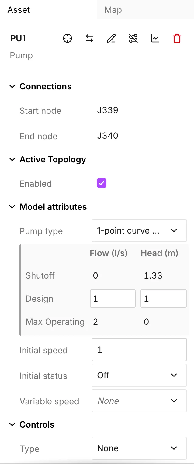
Give the pump placeholder values, so that it does not fail the attribute check. Set Pump type to 1-point curve (design point), with a flow of 1 and a head of 1. Set Initial status to Off. The pump is off because the tank starts nearly full, and because you have not sized the pump yet. Part 5 deals with both.
Proximity check
Section titled “Proximity check”Proximity check lists nodes that sit within a set distance of a pipe they are not connected to. These are the undershoots and the overshoots that a digitizing session leaves behind. Distance at the top sets the radius, and the list recomputes as you change it.
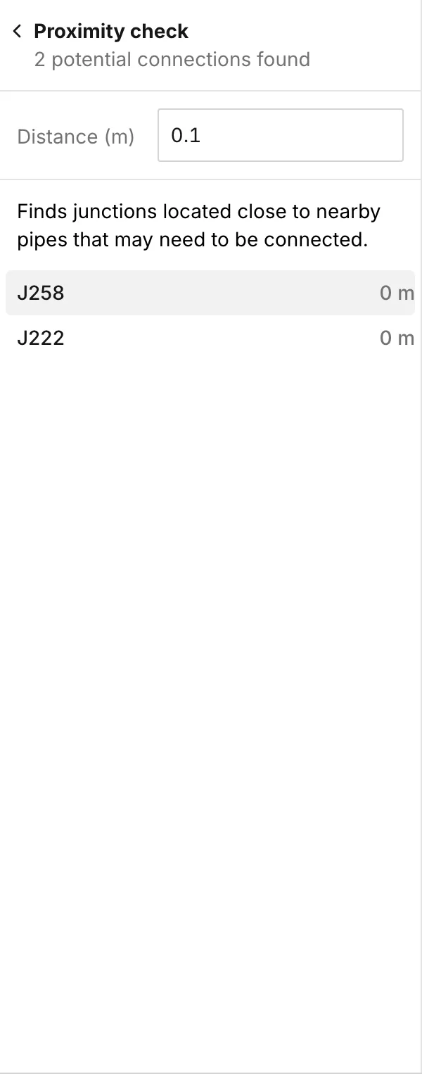
Start at 0.1 m and widen from there. When you select a row, the map frames the node and the pipe and zooms in tight on the gap. That view is what you need to judge the row. To connect the node, drag it onto the pipe. The drag splits the pipe and joins the two in one gesture, and Connect on the row does the same in one press. To leave the node alone, move to the next row.
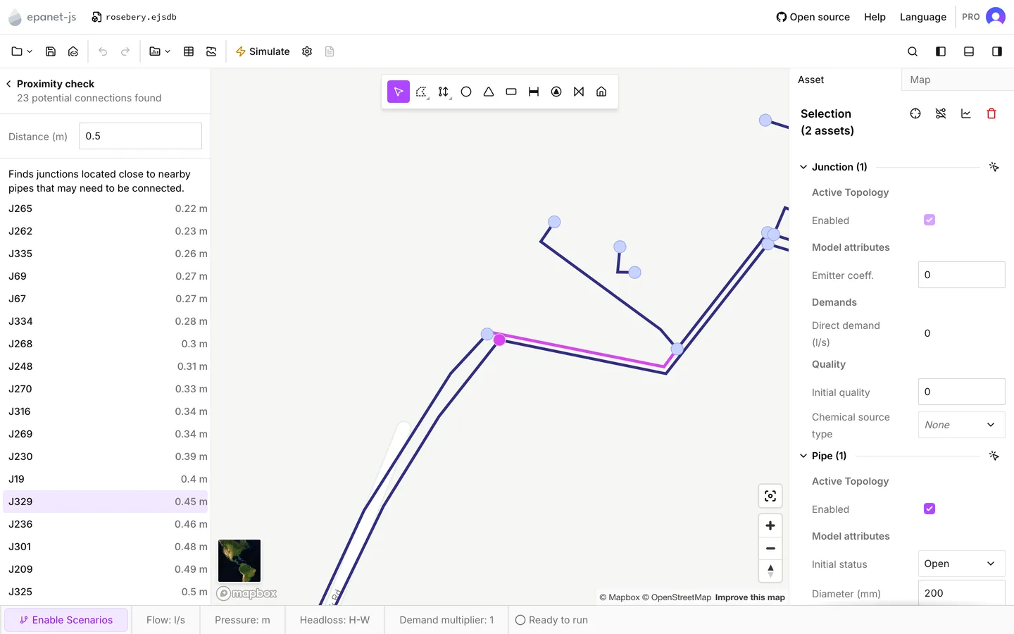
Do not connect every hit. One hit in Rosebery is a service that runs beside the rising main. It is close enough to be reported, and it is not meant to join the rising main. Archive on its row sets it aside under the Archived header, and the count no longer includes it.
Crossing pipes
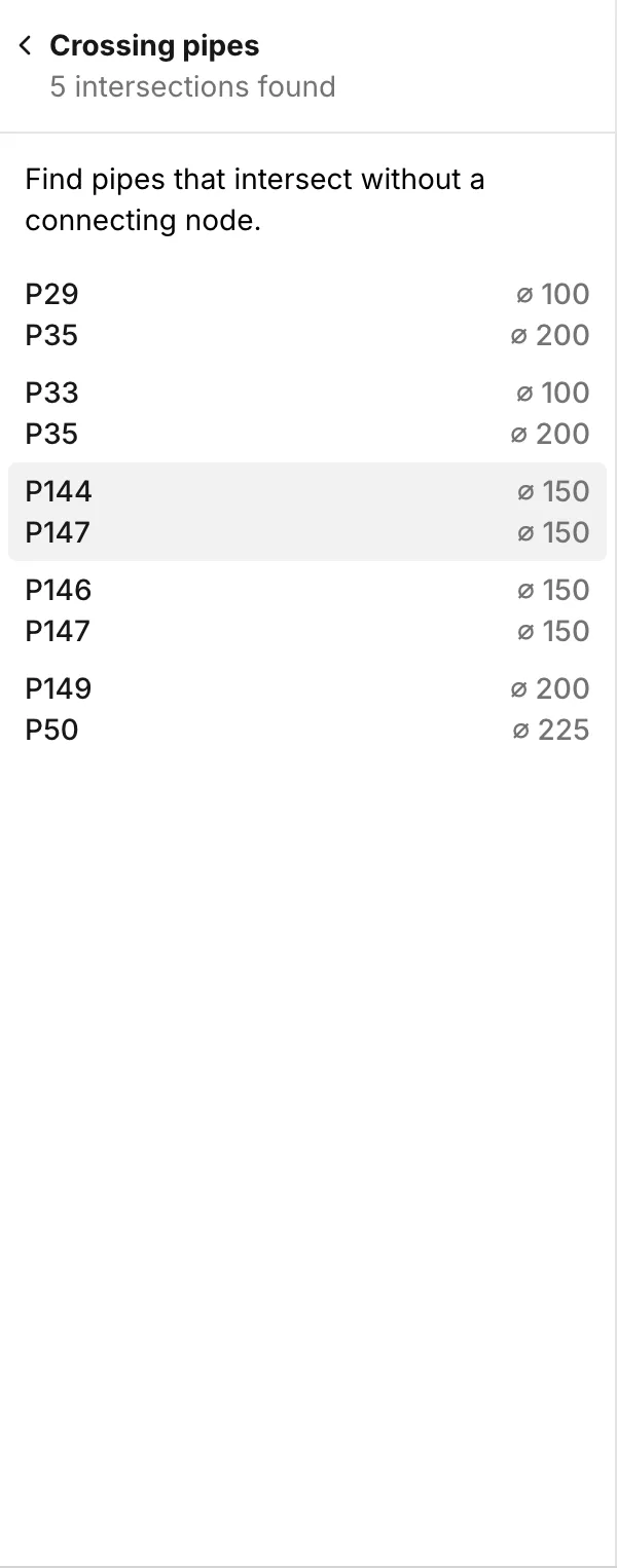
Section titled “Crossing pipes”Crossing pipes finds pairs of pipes whose lines intersect with no node between them. A pair can be a four-way connection that lost its node, or one main that passes over or under another. Nothing in the source data says which, so you judge each row against its two diameters and the basemap underneath. This build connects none of them.
The tank
Section titled “The tank”The builder gives the tank its elevation and nothing else, and a tank with no
shape has no volume. To select the tank, press ⌘+K and
type RSBWS02-004. Then fill in the geometry from what you can see and what the
utility told you.
On the satellite basemap, this tank is a circle about 25 m across. It stands on the ground, not on a tower, and it is about 5 m tall. So set Tank geometry to Circular, Diameter to 25, Min level to 0, Max level to 5, and Min volume to 0. The app computes Max volume from those values, and it comes out at about 2,450 m³.
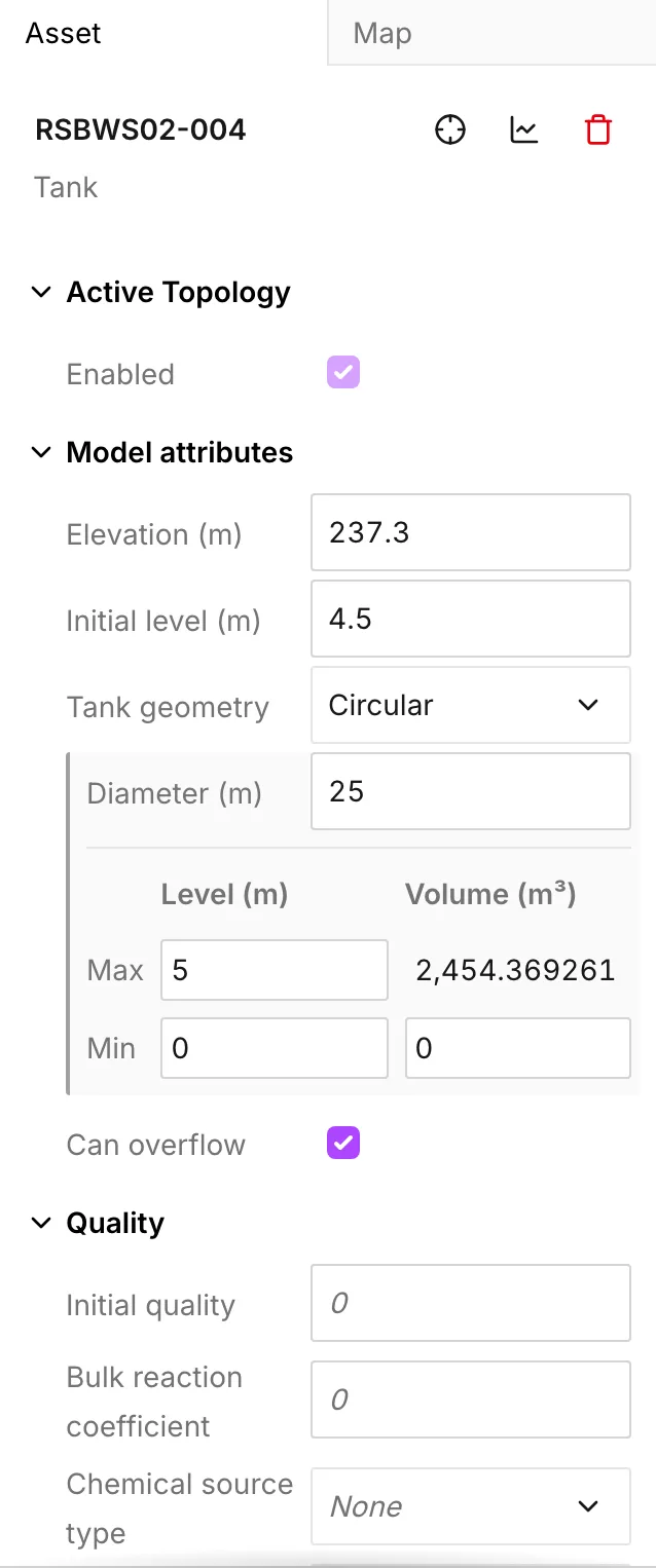
Initial level arrived empty, like the rest of the geometry. Set it to 4.5 m. That leaves the tank nearly full, which is the state the pump must be sized to hold.
See Tanks for the rest of the panel.
The reservoir
Section titled “The reservoir”The build leaves the reservoir’s Head empty for the same reason, and Model attributes reports Reservoir head missing until you set it. Select the treatment works, whose elevation came in at 162.7 m, and set Head to 172.7 m. That value treats the works outlet as if it holds about ten meters of water above the site. The pump in Part 5 is sized against that head. See Reservoirs.
Roughness
Section titled “Roughness”Open Data tables from the toolbar. Tick Pipes and press Open. Every row has a Material and a Year of installation. Roughness is empty on every row. The extract never had a roughness, and Hazen-Williams will not run without one.
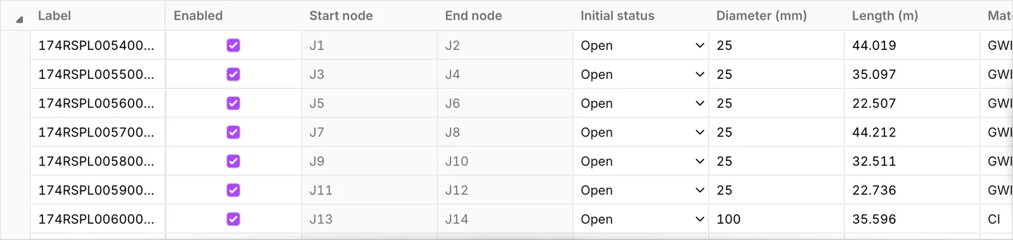
Typing 348 numbers is not the answer. The pipe library holds one roughness for each material at each age. A pipe with a material and a year takes its roughness from the library, and you type nothing on the pipe itself.
-
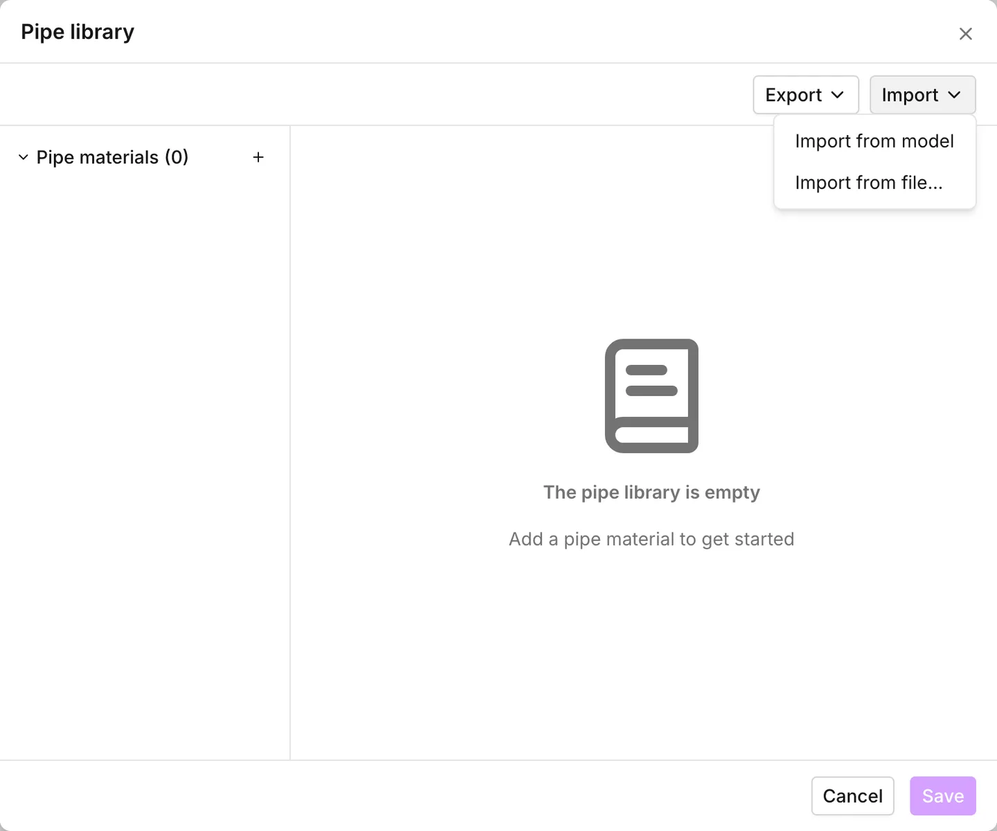
Open Operational data > Pipe library, then choose Import > Import from model.
-
What arrives is the shape of the table and none of its content. Every distinct Material on the pipes becomes a material in the library. Each material gets one entry for each decade of pipe age in the model, all at the default roughness.
For Rosebery, the list runs from
ACandCIthroughPVC,PVC-OandPE100. The ages come in two clusters: mains laid about 1960, and mains laid since 2016.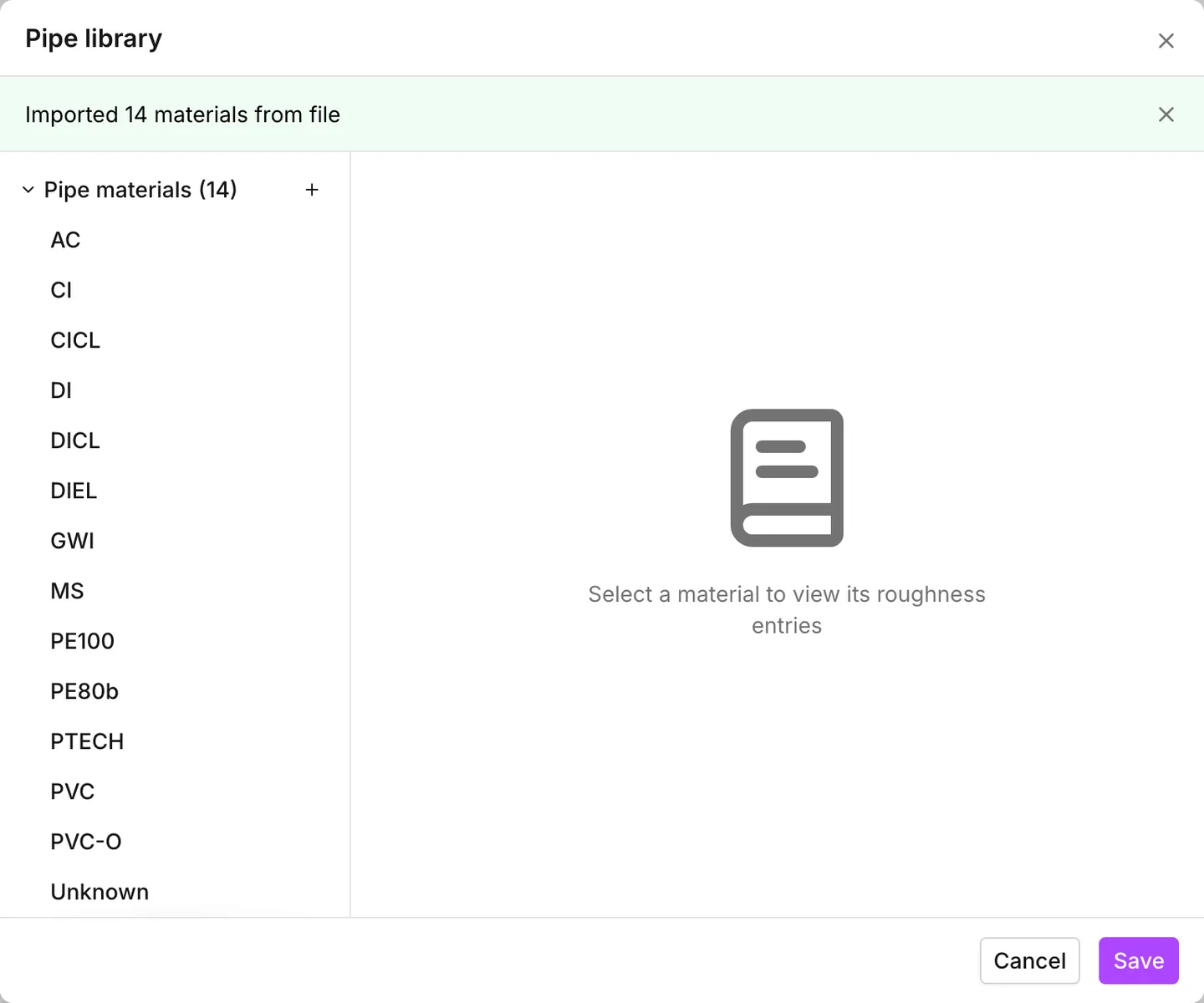
-
Select each material and set its Roughness against Age. These values are C-factors, because the project is on Hazen-Williams. Use about 130 for the asbestos cement and the older cast iron. Use more for the plastics, which are newer and smoother. To fill the table in a spreadsheet instead, press Export. It writes the table as a
.csvor an.xlsxfile, and you import it back.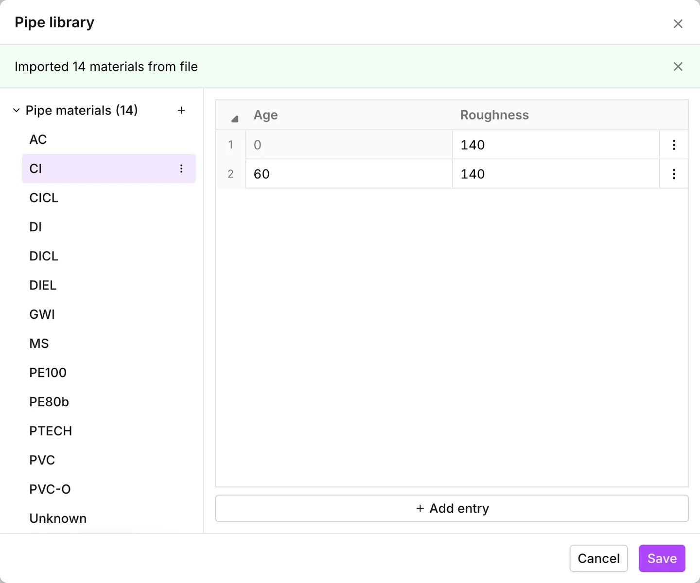
-
Press Save. Every pipe whose material the library names now shows a roughness in italics. That value belongs to the library, and it stands in as a placeholder. The run and the export use it exactly as they use a typed value. When you type over it, the value becomes the pipe’s own. When you delete what you typed, the pipe goes back to the library value.
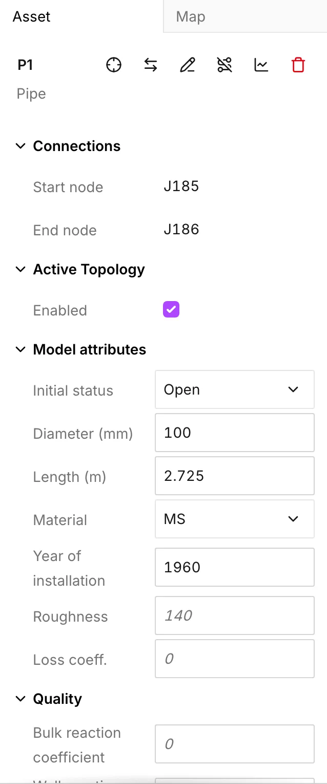
Two kinds of pipe are left out, and Model attributes in Network Review names both.
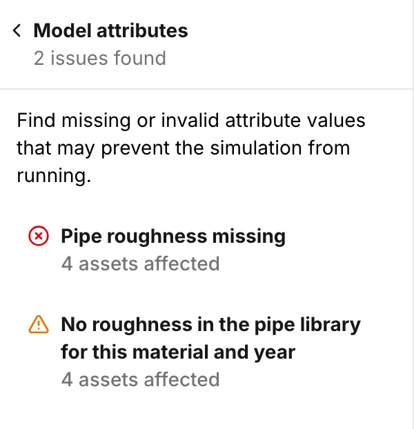
- Pipes with a material and no year. A material with several age entries needs
the year to choose between them, and with no year it gives nothing. Some of
the
PVCandPVC-Omains have no install date. Delete the extra rows from those materials until one entry is left. A material with one entry applies at any age. - Pipes whose material is not in the library. Rosebery has a few marked
Unknown. AddUnknownas a material with one entry, and give it 140 as a placeholder. An honest guess is better than a pipe the engine cannot use, and it is one row to come back to.
A run that balances
Section titled “A run that balances”Press Simulate, or Shift+Enter. The run now completes.
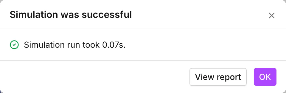
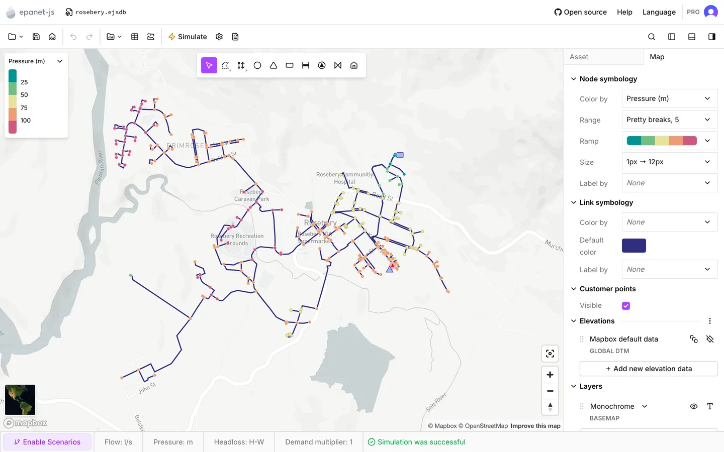
The report balances, and that is the expected result. There is no demand anywhere, so the network has nothing to carry. The flows are zero, so what you read at this point is the pressures. They are the terrain plus the tank level and nothing else. Color the map to see them: Map tab > Node symbology > Color by > Pressure. A pressure that makes no sense points at a connection that went in the wrong place. See Symbology and Reading results.
Part 3 — Demands from the customer layer
Section titled “Part 3 — Demands from the customer layer”The demands for Rosebery are in the customer file. It holds 665 metered
connections that carry avg_demand, about 678,000 liters a day between them.
That is about 7.8 L/s averaged over the day.
Import the points
Section titled “Import the points”File > Import > Customer points.
-
On Data input, drop in
customers.geojson. The import wizard reads the file and moves on by itself, so there is nothing to press here. If the model already has customer points, the import replaces all of them. It warns you first and offers Delete and import.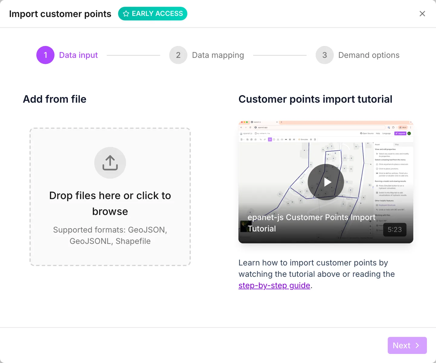
-
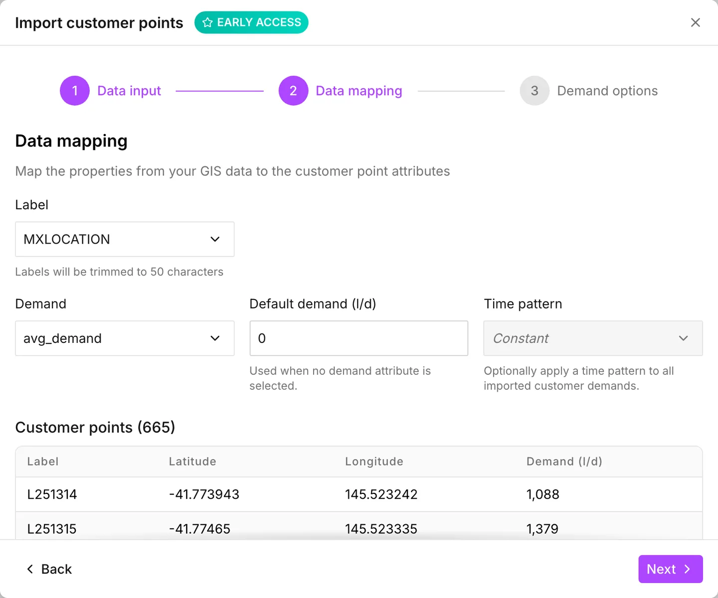
On Data mapping, under Attributes mapping, set Demand to
avg_demandand Label toMXLOCATION. The table under the mapping shows what the import creates. Customer demands are read per day, so in metric unitsavg_demandis liters per day. On a project in US units, the app reads the same field as gallons per day.Default demand is what a point gets when the attribute is missing or unreadable. If you set Time pattern, every point gets that pattern as it lands. Leave it empty. A pattern goes on later, once there is a run to justify its shape.
-
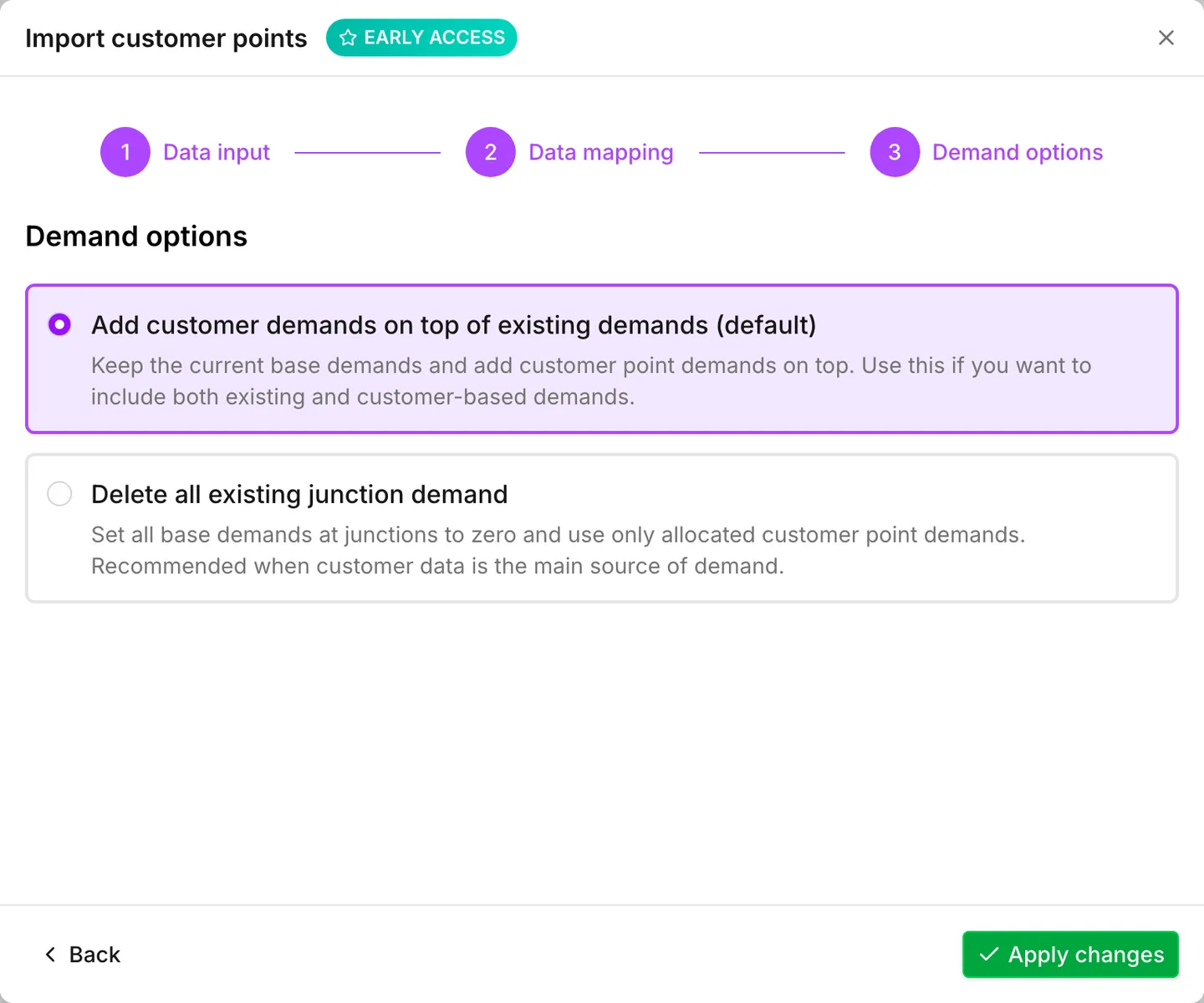
On Demand options, the model has no junction demands yet, so the choice makes no difference here. Choose Add customer demands on top of existing demands (default), then press Apply changes. That ends the import. The model now holds 665 customer points, and none of them is attached to a pipe yet.
Attach them to the network
Section titled “Attach them to the network”The points attach to pipes in a step of their own, with a dialog of its own. Allocate customer points in the toolbar opens it. Allocation rules cap how large a pipe a customer can connect to, and how far the connection can go. The summary underneath counts how many points the current rules place, before you commit to them.
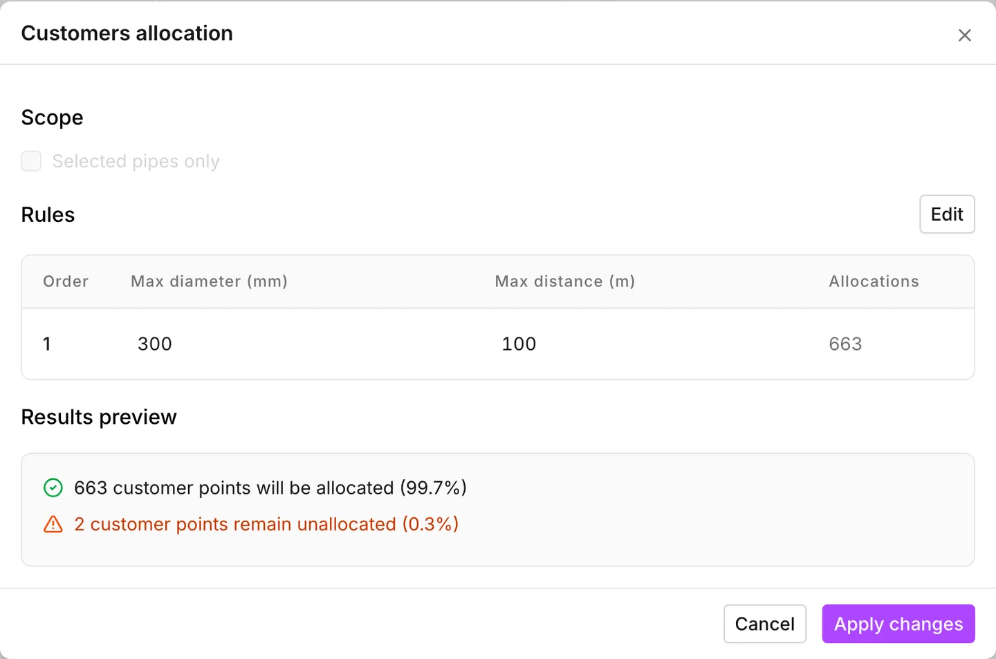
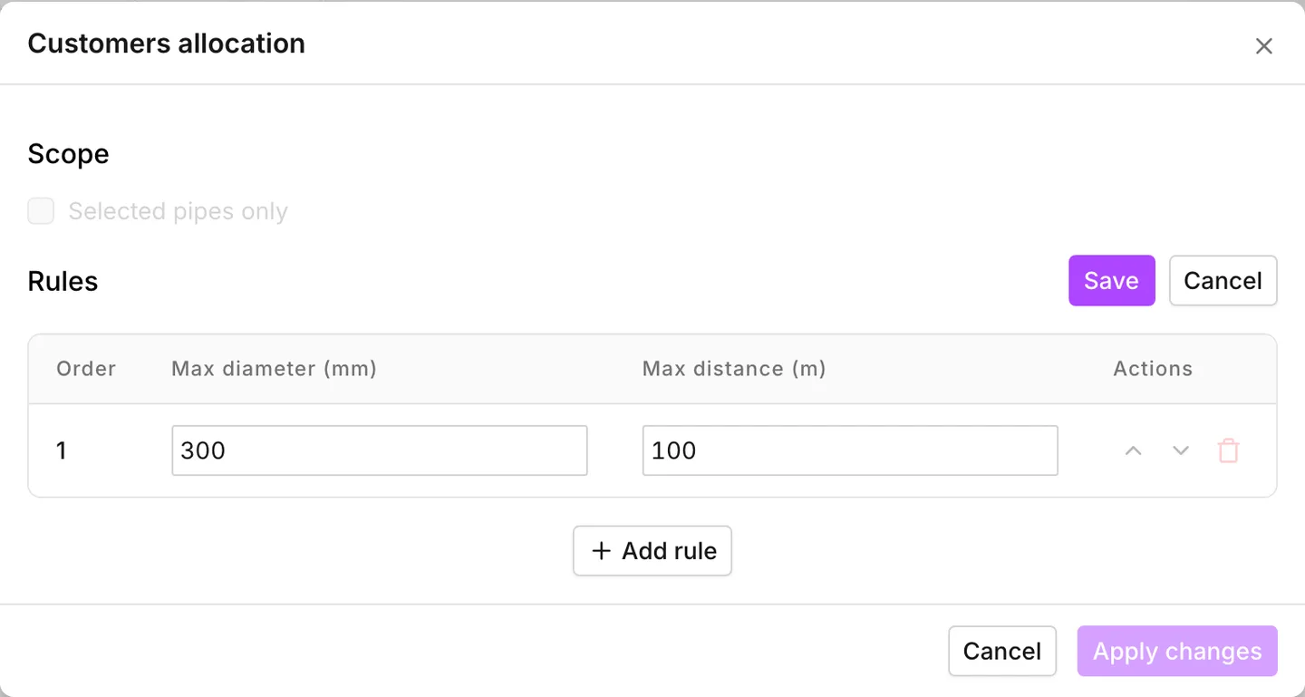
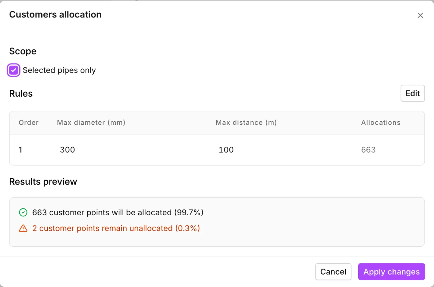
The single default rule in metric units is Max diameter 300 and Max distance 100. Rosebery has a few properties further from any main than that, so the summary comes up short. Press Edit and raise Max distance until nothing is left over. Then press Save.
With Add rule you can add a second, narrower rule instead. The app tries the rules in order, so a tight rule over a loose one gives priority to short connections on small mains.
With every point allocated, press Apply changes.
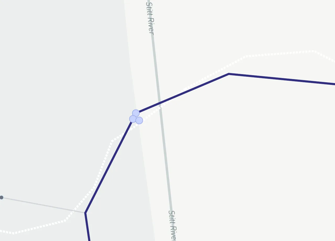
Zoom in, and each customer point is drawn against the pipe it attached to. The nearer of that pipe’s two end junctions carries the demand. Where the other end is the tank or the reservoir, the one junction carries it. The Connected customers field on a pipe lists the customers on that pipe with their demands.
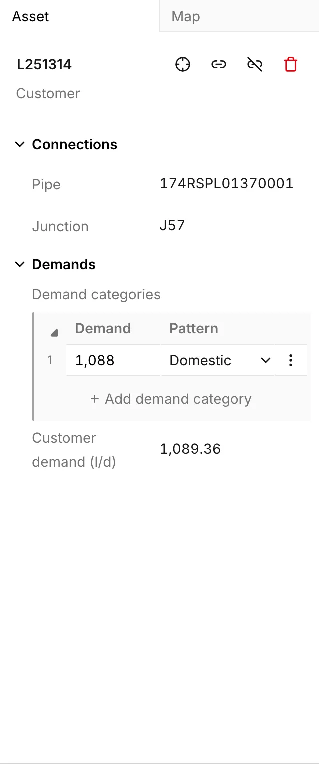
Select a customer point, and the panel names its Pipe and its Junction. If the point attached to the wrong main, Reconnect (Shift+C) attaches it to the pipe nearest the pointer. Hold Shift to aim at a particular point along a pipe. See Customer points.
Allocating a second time, on a selection
Section titled “Allocating a second time, on a selection”Allocation is not only an import step. Allocate customer points in the toolbar opens the same dialog again, on the model as it stands. You can limit the allocation to the pipes you selected, which is how you keep customers off a main they must never be on.
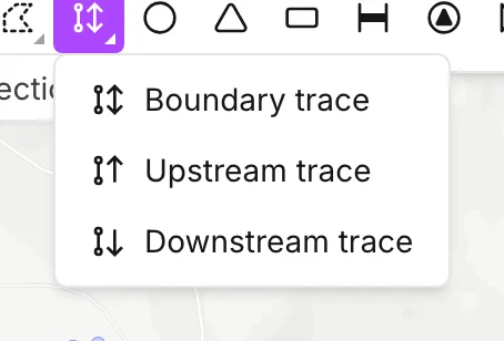
The rising main is that case here. It runs from the treatment works to the tank, past properties that are fed from the distribution network and not from the rising main. Take the Selection trace tool, and right-click it for Boundary trace. That menu belongs to the toolbar button, not to the map. Then click anywhere in the distribution network. The trace stops at the tank, so what you get is the distribution network without the rising main.
Then open Allocate customer points and tick Selected pipes only under Scope. The summary recounts against the selection. Press Apply changes.
Run it
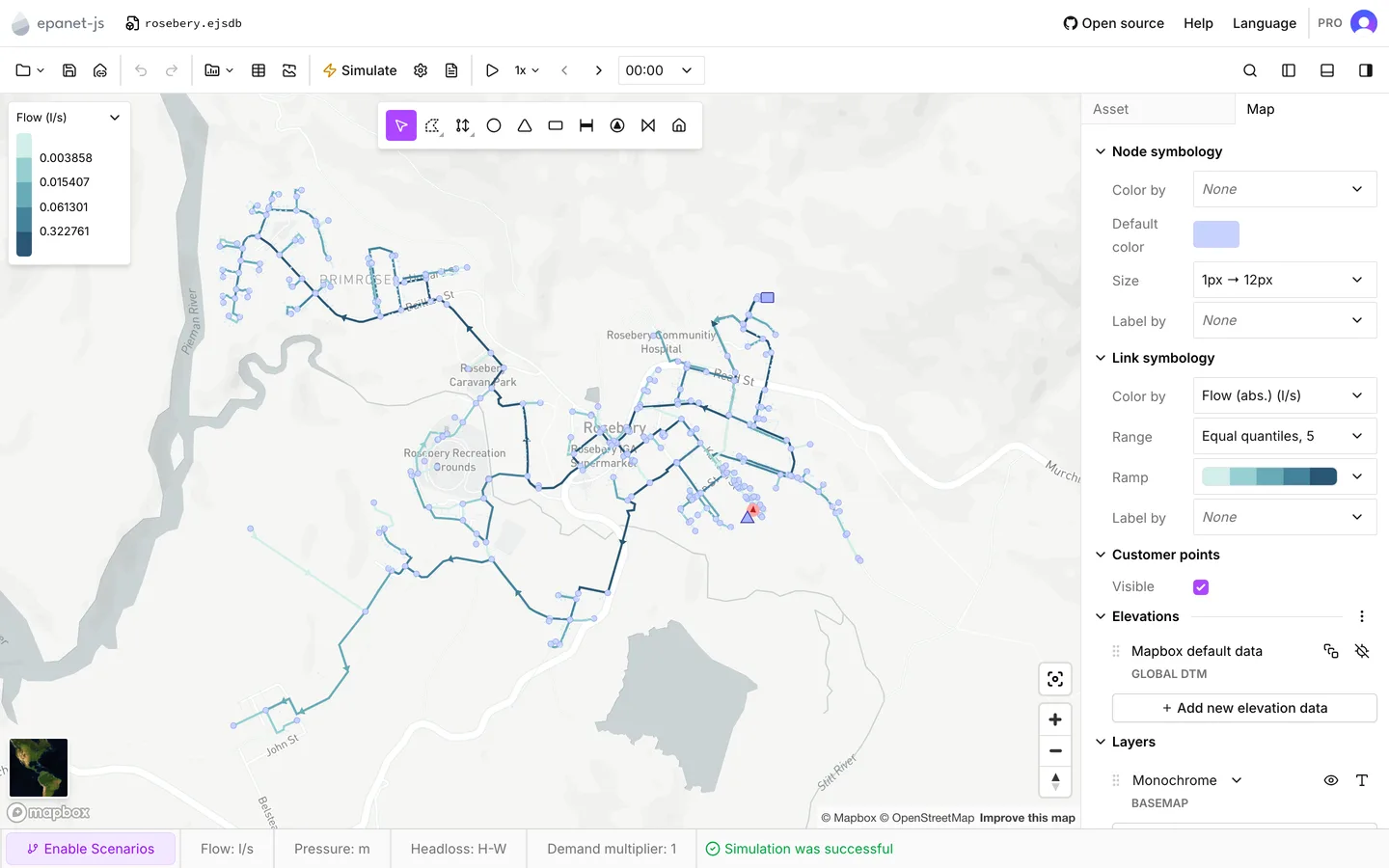
Section titled “Run it”Press Simulate again. The run is still a single steady state, one average moment, but now there is water moving in it. Color the mains by flow: Map tab > Link symbology > Color by > Flow. Select any pipe to read the value.
Part 4 — Twenty-four hours
Section titled “Part 4 — Twenty-four hours”-
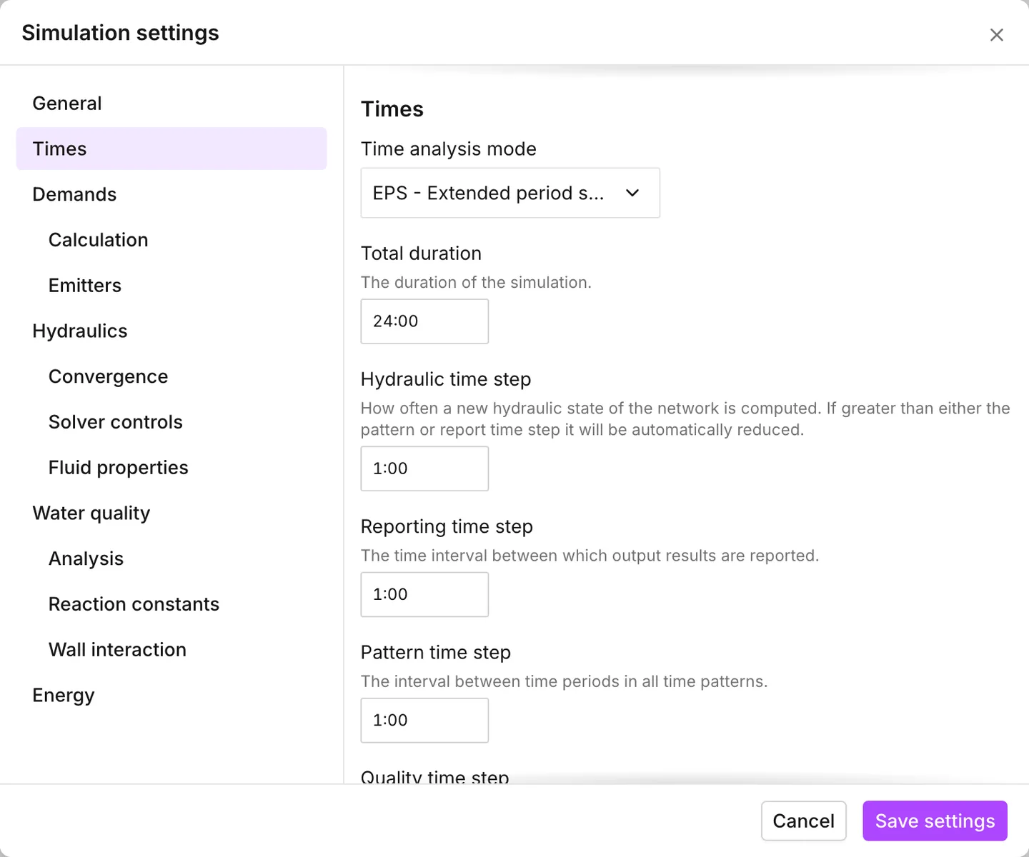
Press Alt+E, or open Simulation settings from the toolbar. In Times, set Time analysis mode to EPS - Extended period simulation. The defaults that appear are a Total duration of 24 hours, with hourly reporting and pattern steps. This build wants those defaults. Press Save settings.
-
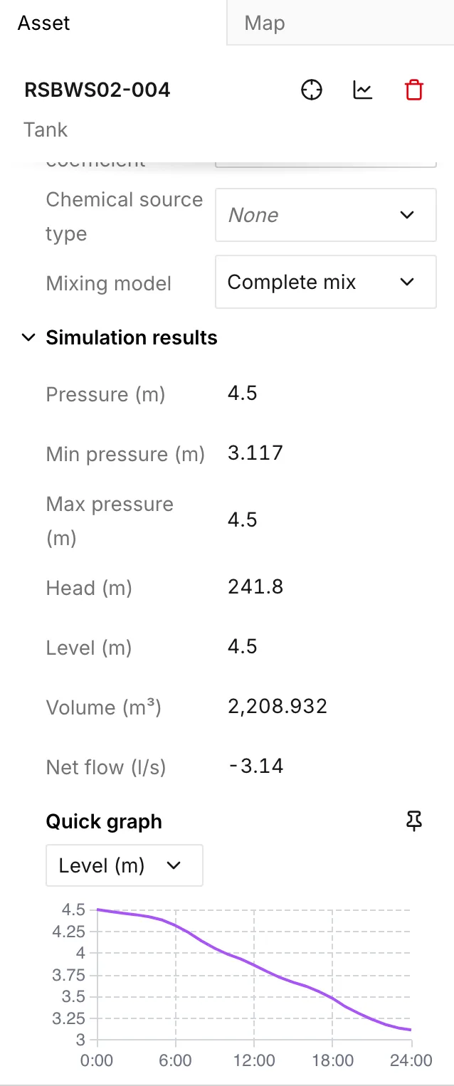
Run the model. Two things appear that were not there before. The time browser in the toolbar steps you through the results. Quick graph at the bottom of the Asset tab graphs the selected asset over the run.
Select the tank. It drains steadily and does not stop, because the pump is off. Select a junction, and its pressure is a flat line, because you gave it the same demand at every hour.
-
Give the demand a shape. Open Operational data > Patterns, then Add Demand pattern, and set Pattern name to
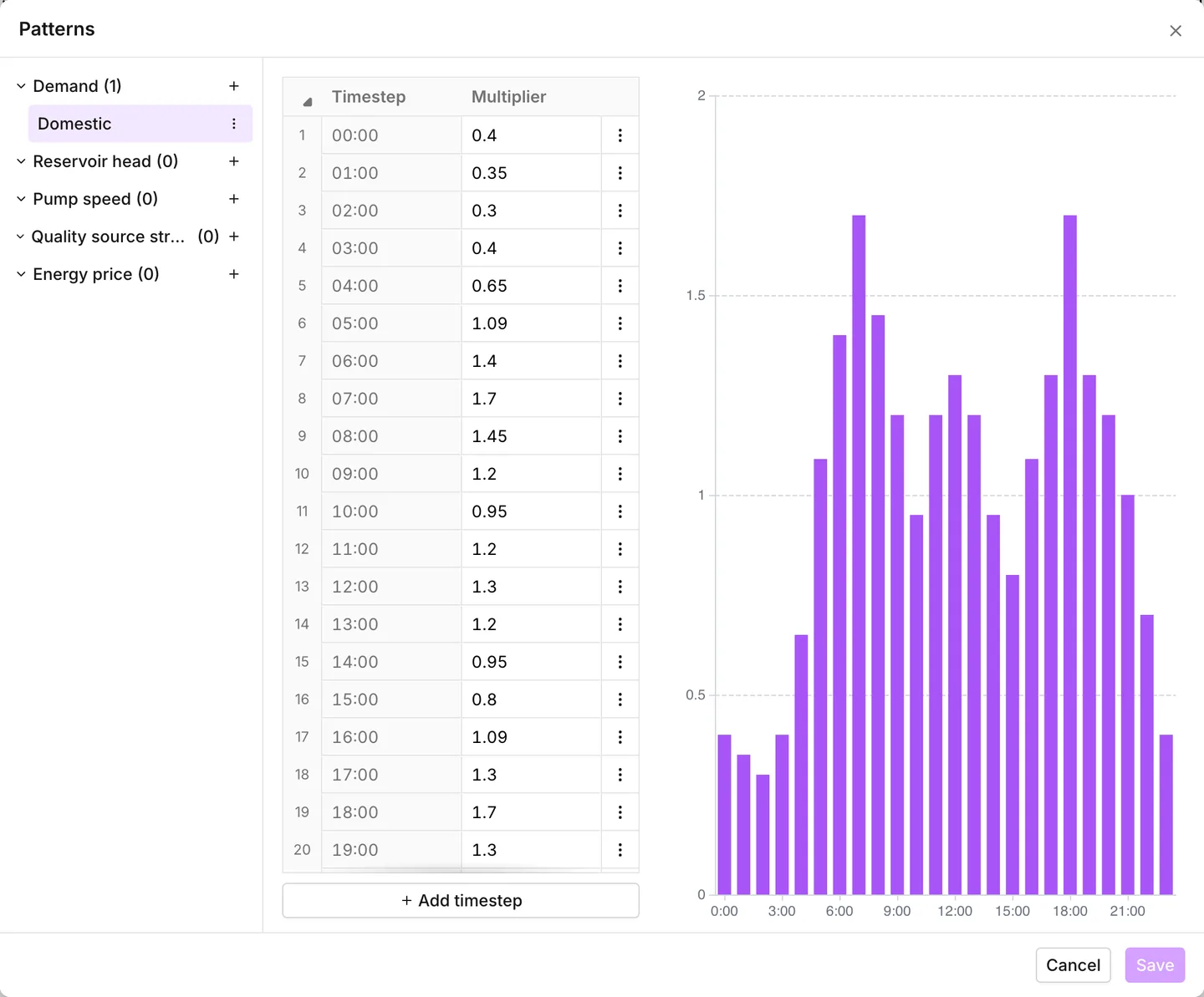
Domestic. The table takes a paste, so copy the column from the table that follows instead of typing it.Hour Multiplier Hour Multiplier 00:00 0.4 12:00 1.3 01:00 0.35 13:00 1.2 02:00 0.3 14:00 0.95 03:00 0.4 15:00 0.8 04:00 0.65 16:00 1.09 05:00 1.09 17:00 1.3 06:00 1.4 18:00 1.7 07:00 1.7 19:00 1.3 08:00 1.45 20:00 1.2 09:00 1.2 21:00 1 10:00 0.95 22:00 0.7 11:00 1.2 23:00 0.4 The pattern has two peaks of about 1.7, one in the morning and one in the evening, on each side of a daytime plateau. That is a domestic profile for a town with no large industrial user on it. The number of rows in the table follows Total duration and the pattern time step. There are 24 rows here, because you set 24 hours at hourly steps. Press Save.
-
Put the pattern on the customers. Open Data tables from the toolbar. Tick Customer points and press Open. Set the Pattern cell on the first row to
Domesticand copy it with Ctrl+C. Click the Pattern column header to select the whole column. Then paste. A single copied cell repeats down the whole selection, so all 665 points take the pattern in one step and one undo.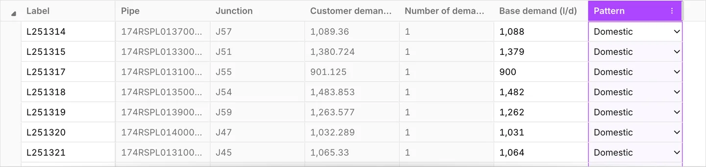
-
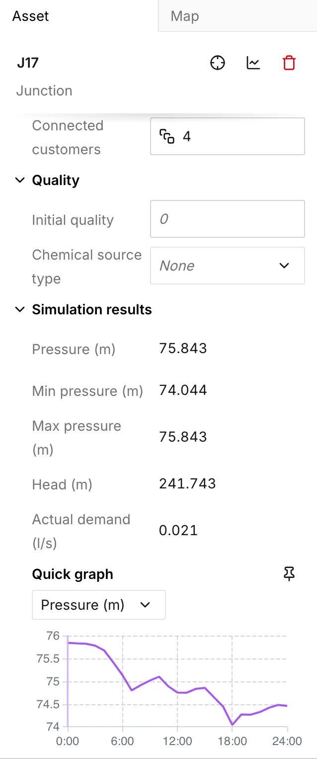
Run again. Flow now varies through the day. The Quick graph of a junction shows the pressure dip at the peaks and recover overnight, with the tank level under it. The head at every junction below the tank moves with the tank level. Pin keeps a graph on screen while you select other assets. See Graphs.
Part 5 — Size the pump, then control it
Section titled “Part 5 — Size the pump, then control it”With the pump off, the tank only drains. Two things correct that: a pump large enough to refill the tank, and a rule that stops the pump once it is full.
Size it
Section titled “Size it”The two numbers come off the model you just ran.
- Head. The tank floor is at 237.3 m and you gave the tank 5 m of water, so a full tank is at 242.3 m. The head you gave the reservoir is 172.7 m. The difference is about 70 m. At these flows, the friction in the rising main is small beside that difference.
- Flow. Average demand over the day is about 7.8 L/s. A pump at 10 L/s refills faster than the town empties, and that is what lets the pump run in cycles instead of continuously.
Select the pump, keep Pump type on 1-point curve (design point), and put 70 m of head against 10 L/s in place of the placeholder. Set Initial status to On.
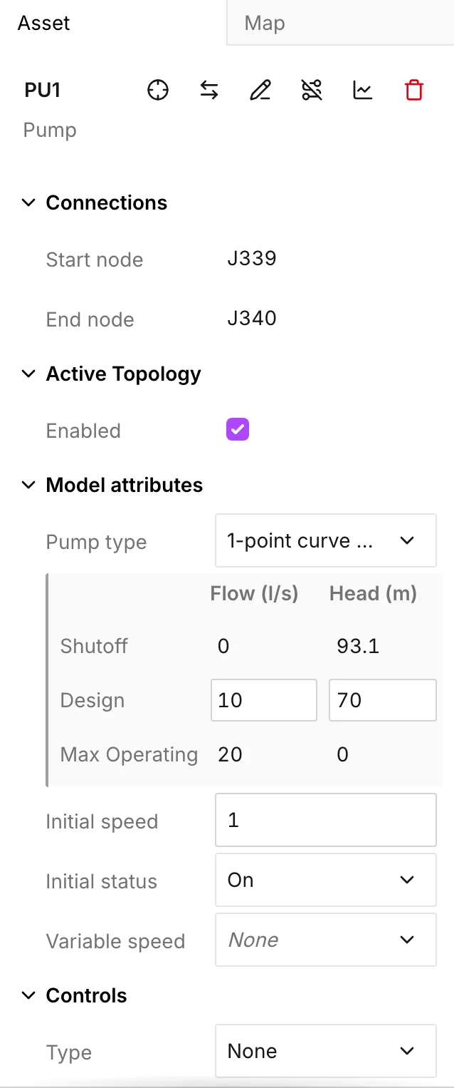
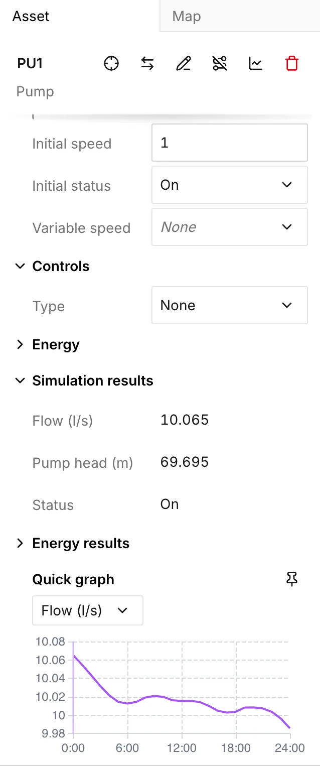
Run the model. The pump delivers about 10 L/s and the tank fills. It then goes on filling, because nothing tells the pump to stop. On the Quick graph of the pump you can watch the operating point move. As the tank fills, the head the pump works against rises and the flow falls away. See Pumps.
Control it
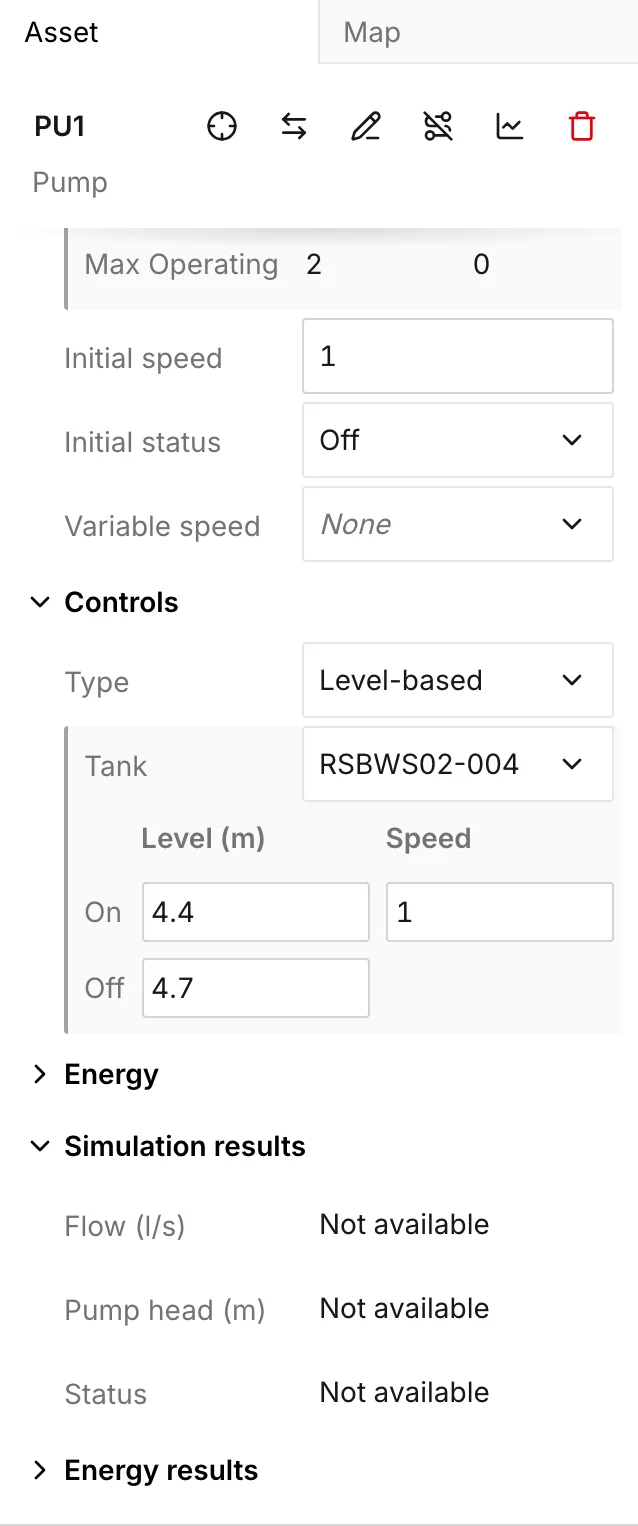
Section titled “Control it”Switch the pump on below one tank level, and off above another. In the Controls section of the pump panel, set Type to Level-based and choose the Tank. Then give the two rows their levels: on at 4.4 m at full speed, and off at 4.7 m. The on level must be less than the off level. Both levels must lie between the tank’s Min level and Max level.
Native controls are a paid feature. Without them, write the same thing as EPANET control statements. Press Alt+C, or open Operational data > Controls. Take the Simple tab of Legacy EPANET controls, and write one statement per line.
LINK PU1 1 IF NODE RSBWS02-004 BELOW 4.4LINK PU1 0 IF NODE RSBWS02-004 ABOVE 4.7PU1 is the label the app gave the pump when you drew it, because pumps are
numbered PU1, PU2 and so on. RSBWS02-004 is the MXLOCATION of the tank,
which became its label because you mapped ID to it. Use the labels your own
model has. Do not control the same pump in both places. See
Controls.
Three days
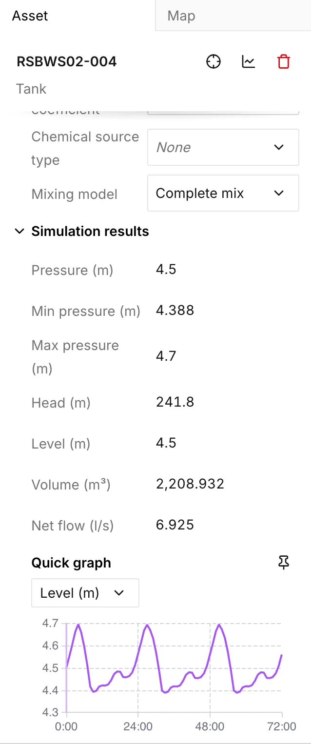
Section titled “Three days”One cycle is hard to read. Raise Total duration to 72 hours and run again. The tank level saws between the two thresholds, the pump starts and stops with it, and pressures across the town cycle with the tank. Three days is enough to show whether the two levels are spaced sensibly. Levels too close together make the pump chatter. Levels too far apart let the tank run low before the pump starts.
Select the tank and a pipe together, and the app graphs both at once. That is the quickest way to see the flow of the pump against the level that drives it.
Press Save, or Ctrl+S / ⌘+S, and
choose where to put the file. The first save tells you
Your work is now saved as a Project and writes an .ejsdb file. That is the
project format, and it keeps everything you built, including the customer
points, the pipe library and the native control. The file goes to your own disk.
Nothing is uploaded, and the run itself also happens in your browser. See
Projects.
The next section needs an INP. To write one, use File > Export > EPANET INP. An INP is the EPANET format and not the format of this app, so some of what you built has no place in it. The app says what those parts are before it writes the file. See Importing and exporting.
Fire flow across the whole network
Section titled “Fire flow across the whole network”The last part uses a separate application. Help > Utility apps opens
utils.epanetjs.com, a companion site of EPANET tools. One of those tools runs
a fire flow analysis over every junction in a model at once.
Give the tool the INP you exported. It asks for three things: the hour of the
run to test, a fire flow rate to target, and a minimum residual pressure. Take
07:00, the peak of the Domestic pattern. A rate of 15 L/s and a pressure of
5 m suit this network. Then run the tool for all junctions.
It reports, per junction:
- Available fire flow. This is the most the network can deliver there before the pressure falls to your minimum. If the minimum is 20 m and the tool reports 86 L/s, then 86 L/s is what the junction can give.
- Needed fire flow. Where the target is less than the available flow, the tool runs again at the target and reports the residual pressure that is left.
A junction fails for one of two reasons. Its starting pressure is already less than the minimum, or the network can supply something but not the target. Results come back as a colored map and a table, and the two are linked. When you click an asset, the tool shows its row. When you click a row, the map flies to the asset.
What this covered
Section titled “What this covered”- Importing a network from GIS layers, and mapping the few attributes that matter — see Build a model from GIS.
- Finding and fixing what an extract gets wrong: disconnections, orphans, near misses, crossings and drainage in the mains layer — see Network review.
- Roughness for a whole network from materials and years — see Pipe library.
- Demands from a customer layer, and the rules that decide where they land — see Customer points.
- Steady state to extended period, and a demand pattern pasted down a column — see Settings, Patterns and Data tables.
- A pump sized from the tank it fills and controlled off its level — see Pumps and Controls.
- Saving a project, exporting an INP, and taking that INP somewhere else — see Projects and Importing and exporting.