Simulation settings

Simulation settings holds the EPANET options for the project:

• How long the run is, and at what interval
• How the app calculates demand
• What the engine does when it fails to converge
• Whether the run computes water quality and energy at all

Most models need nothing here beyond the Times section. The rest is there for when a run misbehaves, or when a study needs something other than the defaults.

This page says where each option is, when it is available, and what the app does with it. Each row carries a one-line description in the dialog. For what any of them means to the engine, see the EPANET 2.2 manual.

Opening it

Simulation settings in the toolbar opens the dialog. Alt+E (⌥E on a Mac) opens it too. See Keyboard shortcuts.

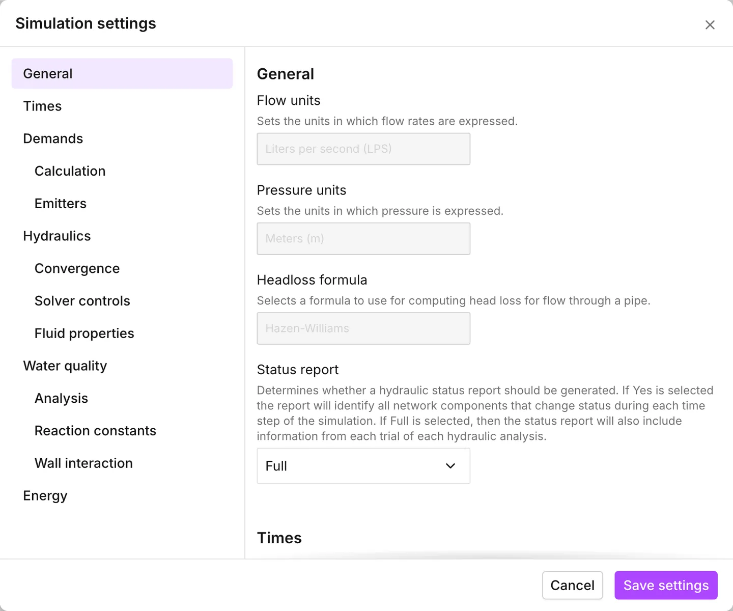
The dialog is one long scrolling form, with a contents list down the left. When you click an entry, the form scrolls to it. When you scroll the form, the highlight moves with it. Nothing is hidden behind a tab. There are six sections, and three of them have subsections:

Section	Subsections	What is in it
General	—	Units, headloss formula, and the status report
Times	—	Steady state or extended period, duration, time steps
Demands	Calculation, Emitters	Demand multiplier, DDA or PDA, emitter behavior
Hydraulics	Convergence, Solver controls, Fluid properties	Trials, accuracy, status checks, viscosity
Water quality	Analysis, Reaction constants, Wall interaction	Which quality analysis runs, and its constants
Energy	—	Pump efficiency, energy price and demand charge

The app applies nothing until you press Save settings. Cancel closes the dialog and discards every change in it without asking. Esc does the same.

General

Three rows are read-only, and grayed accordingly: Flow units, Pressure units and Headloss formula. They are properties of the project, not of the run. You choose them in the New project dialog. The app also reads them from the [OPTIONS] section of an INP when you import one. After that, nothing in the app changes them.

To move a model to different units, import an INP that declares the units you want. The app reads the numbers in an INP as the units that the file itself declares.

The three values are also on the status bar at the bottom of the window, in a shorter form. The bar shows the EPANET code of the formula, H-W, D-W or C-M. This dialog shows Hazen-Williams, Darcy-Weisbach or Chezy-Manning. See The interface.

Status report is the one editable row. It controls how much the run writes into the simulation report:

• No writes nothing.
• Yes writes the components that change status at each timestep.
• Full writes the same, plus every trial of every hydraulic analysis.

Full on a long extended period run produces a very long report. New projects and models built from GIS start at Yes. Both demo networks are saved at Full.

Times

Time analysis mode decides the shape of the run, and everything under it follows from that choice.

• Steady state solves the network once, at the demands as they stand. The six time fields under it are disabled and read N/A.
• EPS - Extended period simulation solves the network again and again over a period. This is what makes patterns, controls and tank levels do anything. The time fields become editable, and the run produces the time series that the time browser steps through.

The two are the same setting as Total duration. A duration of zero is a steady state run. In a new project the duration starts at zero, so a new project opens on Steady state.

Time fields take H:MM, H:MM:SS, or a plain number of hours with a decimal. So 24:00, 24 and 24.0 are the same value, and 1.5 is an hour and a half. The fields show the value back as H:MM.

Field	Starting value	Notes
Total duration	24:00	The length of the run
Hydraulic time step	1:00	If it is longer than the pattern or reporting step, the app reduces it
Reporting time step	1:00	The interval the results are stored at
Pattern time step	1:00	The interval between the points of every pattern
Quality time step	empty	Empty means a tenth of the hydraulic timestep
Rule time step	empty	Empty means a tenth of the hydraulic timestep

The starting values are what the mode switch fills in on a project that never had a duration. A project that has one keeps it.

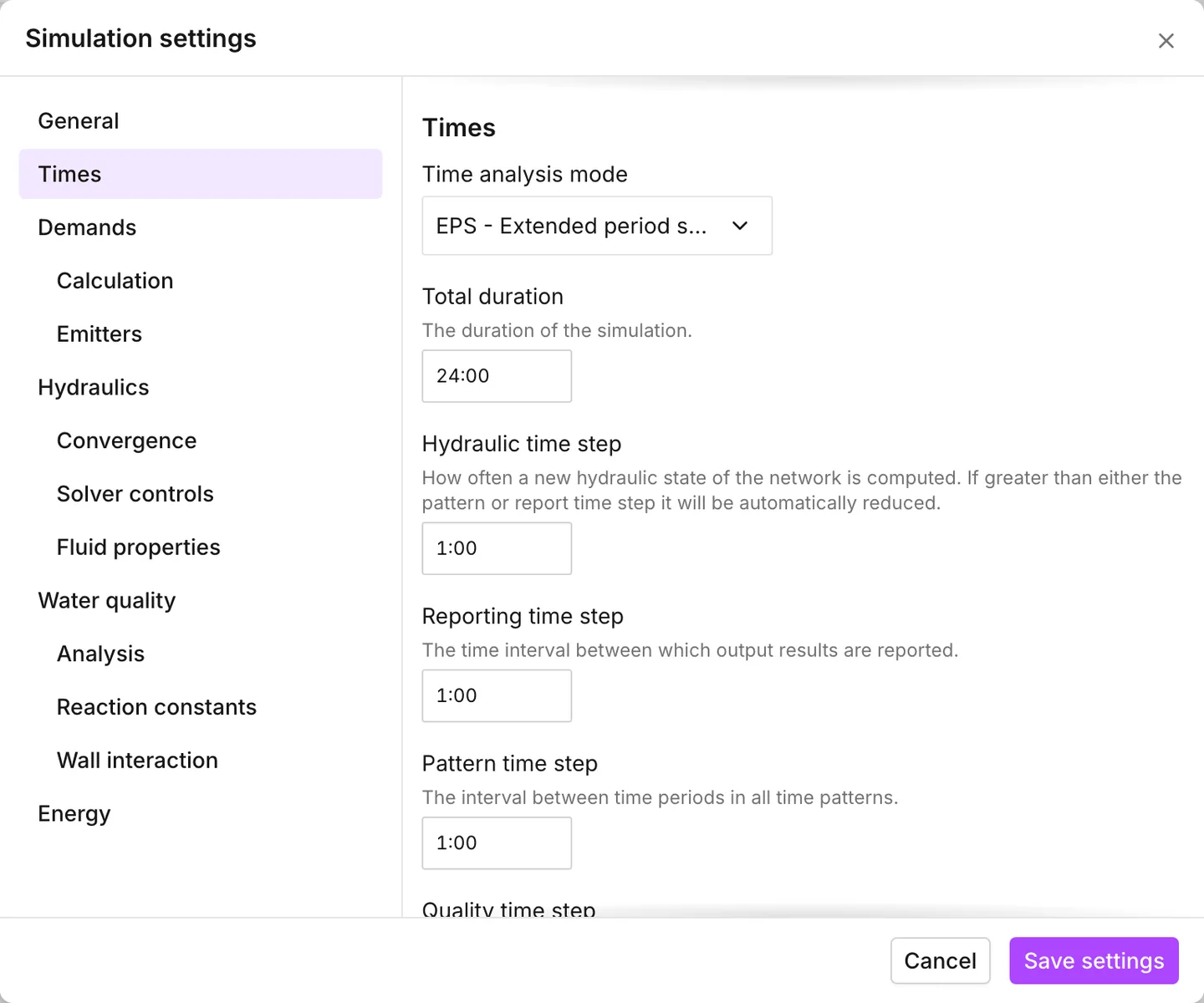
Quality time step and Rule time step are the two that you can leave empty. When they are empty, they show their fallback as a gray placeholder, and the app writes nothing for them. If you clear one of the first four, it takes its stored value back.

When the mode is EPS - Extended period simulation, a 0 in any of the six fields does three things:

• It shows Must be greater than zero beside the field.
• It puts a warning triangle against Times in the contents list.
• It disables Save settings until you correct the value.

Caution

When you switch to Steady state and save, the app stores the duration as zero. The app does not keep the duration you had. When you switch back to EPS - Extended period simulation later, you start at 24:00 again. The other five timesteps survive the round trip. Only the duration is lost.

The pattern timestep is the one to set first on a new model. It is the spacing of the points of every pattern. A 24-point diurnal profile covers a day only when this timestep is one hour. See Patterns.

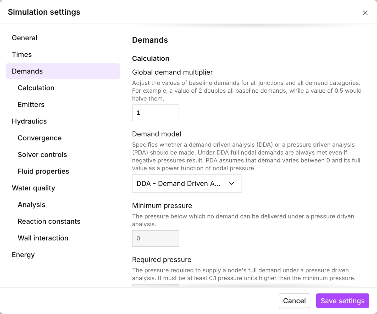
Demands

Calculation holds the five rows that decide how much water each junction takes.

Global demand multiplier scales every base demand at once, on every junction and every demand category. A value of 1.2 gives a 20% growth case. A value of 0.5 halves the demands.

The app never writes the multiplier onto the junctions. The demands on the Asset tab and in the data tables stay as you typed them, and the app hands the multiplier to the engine beside them. Its current value is on the status bar. Without this dialog open, the status bar is the only place that shows a multiplier other than 1. See Junctions.

Demand model switches between two analyses. Under DDA - Demand Driven Analysis, every demand is met, whatever the resulting pressure. Under PDA - Pressure Driven Analysis, the demand delivered varies with pressure. Minimum pressure, Required pressure and Pressure exponent are the three rows that configure this analysis, and they stay grayed under DDA - Demand Driven Analysis.

The dialog does not check these three rows against each other. The required pressure must be at least 0.1 pressure units more than the minimum. This requirement appears in the description of the row and nowhere else, so you find a wrong value only when the run starts.

Emitters has two rows, Emitter exponent and Backflow allowed. They apply to every junction that carries an emitter coefficient. Both are global. The coefficient itself is per junction.

Hydraulics

Nothing in this section changes the network. This section changes how hard the engine tries, and what it does when it cannot get there. These are the settings you use when a run comes back Simulation with warnings and the report says that a system was unbalanced. See Running a simulation.

Subsection	Rows	Default
Convergence	Maximum trials	40
	Accuracy	0.001
	If unbalanced	Stop
	Additional iterations	0
	Max head error	0
	Max flow change	0
Solver controls	Status check frequency	2
	Max status check	10
	Damping limit	0
Fluid properties	Relative viscosity	1
	Specific gravity	1

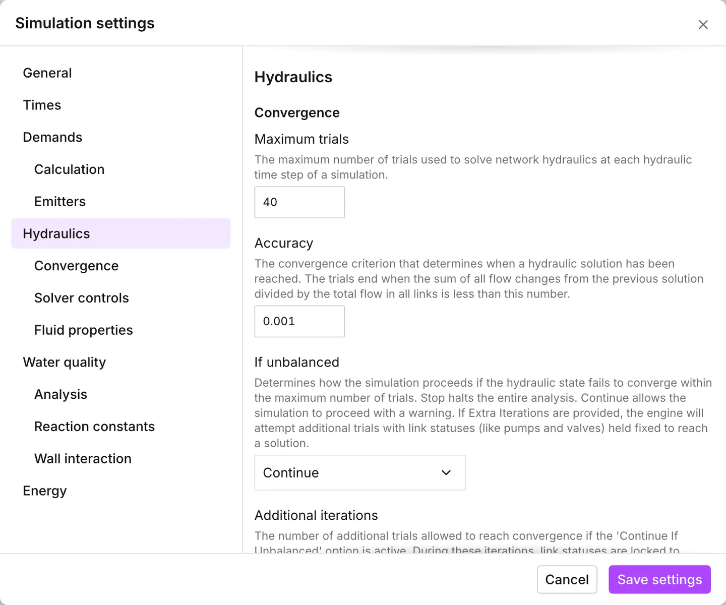
If unbalanced is the row with a visible consequence. Stop ends the run when the trials run out. Continue goes on and reports a warning. Additional iterations is editable only under Continue. It is the number of further trials the engine runs with pump and valve statuses held fixed before it stops. Both demo networks are saved as Continue with 10 additional iterations.

A zero in Max head error, Max flow change or Damping limit means that the criterion is not applied at all. It does not mean that the criterion is set to zero. These rows also accept negative numbers. The dialog checks none of them.

Water quality

Simulation type is the gate for the whole section. It has four choices: None, Chemical, Age and Trace. Everything under it is disabled until you choose one of the last three. Tolerance is then available for all three. Every row in Reaction constants and Wall interaction needs Chemical, and so do Chemical name and Mass unit.

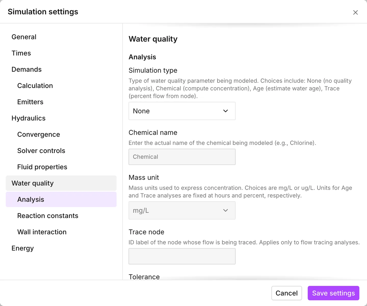
Trace node takes the label of any node: a junction, a tank or a reservoir. The app matches the label without regard to case. A label that is not on a node in this model shows A valid node label is required. It also marks Water quality in the contents list and disables Save settings. So you cannot save a trace analysis without a node to trace from.

Mass unit is the odd one out in this dialog. Its two choices, mg/L and μg/L, are not a simulation setting. They are the concentration unit of the project. A change here also changes how every quality value is labeled on the Asset tab, the data tables and the graphs.

For what each analysis produces, and where the results appear, see Water quality.

Energy

Report energy usage adds a summary of energy and cost for each pump to the simulation report. It is off by default. Four rows under it hold the defaults that every pump uses when it carries nothing of its own: Global pump efficiency, Global energy price, Global energy price pattern and Demand charge. See Pumps and Energy.

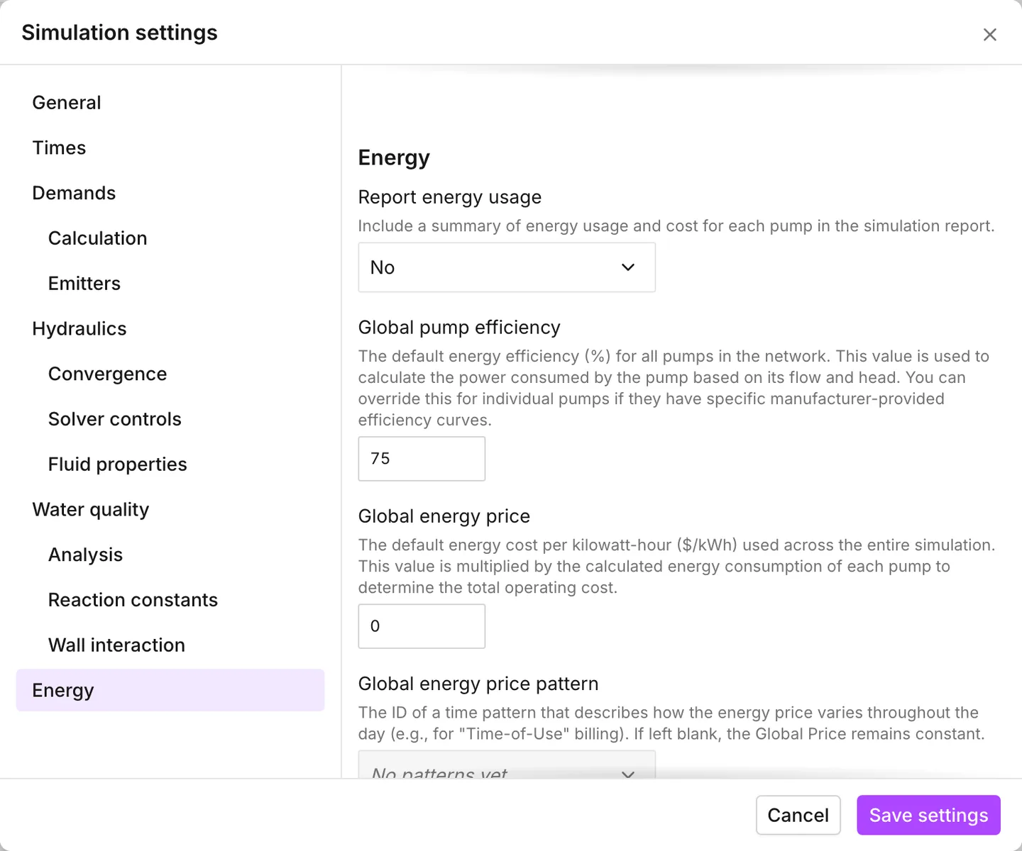
Global energy price pattern lists only the patterns filed under Energy price. When the project has none, the row stays disabled and reads No patterns yet. See Patterns.

Saving

Save settings is disabled in two cases. The first is a time field of zero under EPS - Extended period simulation. The second is Trace chosen with no valid node. These are the only two things the dialog checks. The app hands every other value to EPANET as you typed it. A value that EPANET cannot work with becomes an error when the run starts.

Saving writes straight into the project, so there is nothing more to save for the settings themselves. Two things about it are important:

• You cannot undo a saved change. Simulation settings do not go into the edit history, so Ctrl+Z does not bring the previous values back. If the previous values matter, write them down first.
• Saving invalidates the results on screen. Any completed run becomes Simulation outdated in the status bar, even when your change cannot affect that run.

While a scenario exists

As soon as one scenario exists, every control in this dialog goes read-only, except Global demand multiplier. This happens on every branch you stand on, so that the engine solves every branch with the same settings. To change a run setting, delete the scenarios first. See Scenario work.

What travels in an INP

Almost all of it. An export writes the times, the options, the reaction constants and the energy defaults into [TIMES], [OPTIONS], [REACTIONS], [ENERGY] and [REPORT]. An import reads the same sections back. So a model that leaves as an INP and returns keeps its settings. Two details are important:

• A steady state model writes Duration 0 and no timesteps at all. The timesteps you had are not in the file, so they cannot come back.
• The app writes most of the hydraulics and quality constants only when they differ from its defaults, so an exported file is a short one. A row that is missing from [OPTIONS] is not lost. It is at its default.

See Import and export.

Next

• Running a simulation — the pre-run checks, and what the outcome means.
• Reading results — the time browser an extended period run produces.
• Water quality and Energy — the two sections of this dialog that have pages of their own.
• Patterns — what the pattern timestep spaces out.
• Projects — where the settings are stored.